 |
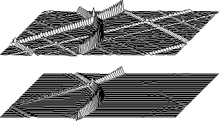
Figure 1 Frequency domain hyperbola (top) and time domain hyperbola (bottom).
![[*]](http://sepwww.stanford.edu/latex2html/prev_gr.gif)
Here we will first look at some general principles having to do with splitting a process into separate, but simpler processes, and how this can be understood by inspecting differential equations. Then we'll look at finite-difference migration in the time domain.
Figure 1 illustrates the differences between Fourier domain calculations and time domain calculations.
 |
The figure was calculated on a 256![]() 64 mesh to exacerbate for display
the difficulties in either domain.
Generally, you notice wraparound noise in the Fourier calculation,
and frequency dispersion
in the time domain calculation.
(The ``time domain'' hyperbola in Figure 1
is actually a frequency domain
simulation--to wrap the entire hyperbola into view).
In this chapter we will see how to do the time domain calculations.
A more detailed comparison of the domains is in chapter
64 mesh to exacerbate for display
the difficulties in either domain.
Generally, you notice wraparound noise in the Fourier calculation,
and frequency dispersion
in the time domain calculation.
(The ``time domain'' hyperbola in Figure 1
is actually a frequency domain
simulation--to wrap the entire hyperbola into view).
In this chapter we will see how to do the time domain calculations.
A more detailed comparison of the domains is in chapter ![[*]](http://sepwww.stanford.edu/latex2html/cross_ref_motif.gif) .
.
Even if you always migrate in the frequency domain, it is worth studying time domain methods to help you choose parameters to get a good time domain response. For example both parts of Figure 1 were done in the frequency domain, but one simulated the time domain calculation to get a more causal response.
Much of seismology amounts to measuring time shifts. The word stepout denotes a change of travel time with a change in location. Frequency-domain calculations usually conclude with a transform to the time domain to let us see the shifts. An advantage of time-domain computations is that time shifts of wave packets can be measured as the computation proceeds. In the frequency domain it is not difficult to reference one single time point, or to prescribe a shift of the whole time function. But it is not easy to access separate wavelets or wave packets without returning to the time domain.
The upward and downward wavefield extrapolation
filter ![]() is basically
a causal all-pass filter.
(Under some circumstances it is anticausal).
It moves energy around without amplification or attenuation.
I suppose this is why migration filtering
is more fun than minimum-phase filtering.
Migration filters gather energy from all
over and drop it in a good place, whereas
minimum-phase filters hardly move things
at all--they just scale some frequencies up and others down.
is basically
a causal all-pass filter.
(Under some circumstances it is anticausal).
It moves energy around without amplification or attenuation.
I suppose this is why migration filtering
is more fun than minimum-phase filtering.
Migration filters gather energy from all
over and drop it in a good place, whereas
minimum-phase filters hardly move things
at all--they just scale some frequencies up and others down.
![[*]](http://sepwww.stanford.edu/latex2html/prev_gr.gif)