Wave-equation tomography by beam focusing

Localized velocity error

To analyze the interplay between the local and the global objective function, I computed the search directions in the case of a spatially localized slowness error. As for the previous examples, I computed the search directions provided by the gradient of both the local and the global objective functions. Figure 6 shows the slowness error that was assumed for the background slowness model ${s}_{0}$ . In addition to the horizontal average, this figure (and the ones that follow) shows the vertical average in panel c) at the bottom of the figure.

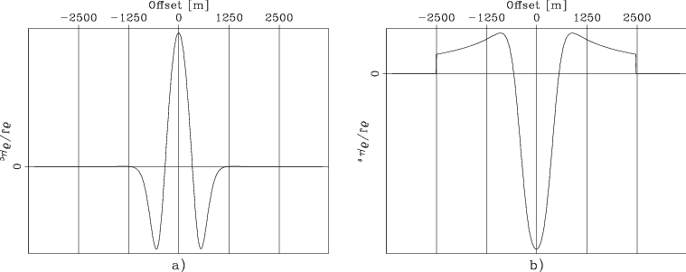
Similarly to Figure 3, Figure 7, shows the derivatives of the objective function with respect to the moveout parameters computed using equations 16-17 and 18-19. The plot in panel a) displays the derivatives with respect to the local curvature, ${\mu _C}$ ; the plot in panel b) displays the derivatives with respect to the time shifts of the beam centers, ${\mu _{\theta }}$ . In both cases the derivatives are plotted as a function of the beam center coordinate, ${\overline {x}}$ , for the source location at $x_{s}=2.56$ km; that is, in the middle of the model. As visible from the figure, I clipped to zero the derivatives for both parameters outside of the $-2.5\; {\rm km} \leq{\overline{x}}\leq 2.5$ km range to avoid edge effects.

Figure 7a clearly shows that local curvature is not as an appropriate parameter for measuring the effects of small-scale velocity errors as it is for large-scale ones. The alternating signs of the objective-function derivatives causes the search direction to be highly oscillating as well. In contrast, the time-shifts derivatives shown in Figure 7b shows a large anomaly corresponding the localized velocity error and will provide useful slowness updates to localize the velocity anomaly.

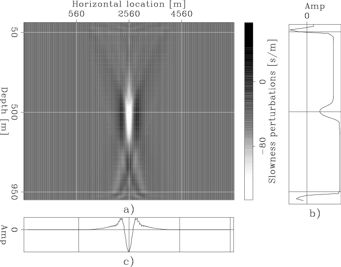
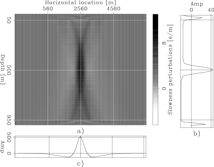
These observations are confirmed by Figure 8 and 9. Figure 8 shows the search direction computed using equation 24. As expected it oscillating around the velocity anomaly. Figure 9 shows instead a nicely localized anomaly with the correct sign. It is useful to notice that the horizontal averages of the search directions shown in Figure 8 and 9 have opposite polarity. The average of the search direction provided by the global component has the wrong polarity, except at the depth of the anomaly. Whereas the average of the search direction provided by the local component has the correct polarity. This observation confirms the analysis that local curvature carries more reliable information for the long-wavelength component of the velocity updates than the global time shifts, as observed when analyzing the uniform velocity error example.

Another interesting observation can be made by computing the ratio between the amplitudes of the slowness updates in the two cases. In the case of uniform error, the update computed from the local curvature is larger than the other by approximately a factor of 200. In contrast, in the case of the localized anomaly, the ratio between amplitudes is only about 10. This difference in relative amplitudes confirms that the two components of the objective function switch in relative importance between the two cases.

Beam-DC-DT-panom Figure 7. Derivatives of the objective functions with respect to the moveout parameters plotted as a function of beam center coordinate, ${\overline {x}}$ , for the source location at $x_{s}=2.56$ km: a) derivatives of ${J_{\rm Local}}$ with respect to to the local beam curvatures, ${\mu _C}$ , b) derivatives of ${J_{\rm Global}}$ with respect to the time shifts of the beam centers, ${\mu _{\theta }}$ .

VH-Avg-Dir-Beam-panom Figure 8. Search direction computed using the gradient of the local objective function ${J_{\rm Local}}$ with the localized velocity error shown in Figure 6: a) slowness perturbations, b) slowness perturbations averaged over the horizontal direction, and c) slowness perturbations averaged over the vertical direction.

VH-Avg-Dir-Glob-Beam-panom Figure 9. Search direction computed using the gradient of the global objective function ${J_{\rm Global}}$ with the localized velocity error shown in Figure 6: a) slowness perturbations, b) slowness perturbations averaged over the horizontal direction, and c) slowness perturbations averaged over the vertical direction.

Wave-equation tomography by beam focusing