|
|
|
|
Wave-equation tomography by beam focusing |
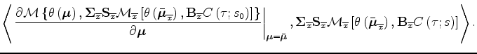
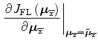
The evaluation of the derivatives of the moveout parameters
with respect to slowness
follows a slightly different procedure from the one above
because the moveout parameters are solutions
of the optimization
problems 5 and 9.
We take advantage of the fact that
we need to evaluate the derivatives only at the solution
points, where the objective functions
are maximized and thus their derivatives with respect to the moveout
parameters are zero.
We can therefore write:
 |
 |
||
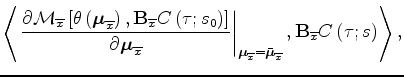 | |||
![$\displaystyle \left\langle
\left.
\frac
{\partial
{
\mathcal M\left\{
{\theta}\...
...ight)
,{\bf B}_{\overline{x}}
C\left({\tau};{s}\right)
\right]
}
\right\rangle.$](img81.png) |
|||
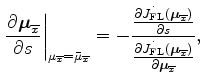
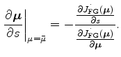
Using the rule for differentiating implicit functions, and taking advantage that the fitting problems are all independent from each other (i.e. the cross derivatives with respect to the moveout parameters are all zero), we can formally write:
Appendix A presents the analytical development of these expressions
to compute the derivatives of the moveout parameters with respect to slowness.
As for the derivatives of the main objective function
with respect to moveout parameters,
the final results for the special case of
![]() and
and
![]() have
a fairly simple analytical expression.
The derivative of the local moveout parameters are
(A-1):
have
a fairly simple analytical expression.
The derivative of the local moveout parameters are
(A-1):
![$ \stackrel{..}{C}\left({\tau}\right)
=
C\left({\tau}\right)\left[
{\widetilde{{P}} }\left({t}\right)
,
{\stackrel{..}{{P}}}_{D}\left({t}\right)
\right]
$](img86.png) .
In both equations 22 and 23
the operator
.
In both equations 22 and 23
the operator
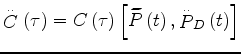 represents a convolution with the recorded data,
whereas the operator
represents a convolution with the recorded data,
whereas the operator
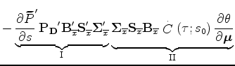
Combining the derivatives in equation 22 with the derivatives in equations 16-17 we can compute the gradient of the local objective function 3 with respect to slowness as:
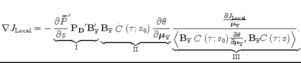 ,
as described by the second term (II).
Notice that the phase introduced by the time derivative
of the correlation function in (II)
is crucial for the successful backprojection into the slowness model
that is accomplished by the first term (I).
In this term, first
,
as described by the second term (II).
Notice that the phase introduced by the time derivative
of the correlation function in (II)
is crucial for the successful backprojection into the slowness model
that is accomplished by the first term (I).
In this term, first
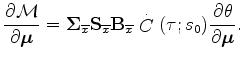
The expression of the gradient of the global objective function 7 with respect to slowness is similarly derived by combining the derivatives in equation 23 with the derivatives in equations 18-19 and is the following three-terms expression:
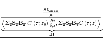 performs the stack over the local arrays and the assemblage
of the stacked traces into the global array,
whereas its adjoint in term I
spreads the stacked traces back into the local arrays
reforming the local beams.
performs the stack over the local arrays and the assemblage
of the stacked traces into the global array,
whereas its adjoint in term I
spreads the stacked traces back into the local arrays
reforming the local beams.
|
|
|
|
Wave-equation tomography by beam focusing |