|
|
|
|
Wave-equation tomography by beam focusing |
To further simplify the theoretical development, I define an objective function that rewards consistency of the correlation computed independently for each source location. The objective function measures correlation consistency along the receiver axis. However, I use here the receiver axis as a proxy for the offset axis or the aperture-angle axis in reflection tomography. The application of the concepts developed in this paper to objective functions useful in reflection tomography should be straightforward, although it will require more complex notation and result in expressions for the gradients even more complex than the ones presented here.
I define the recorded data as
![]() ,
and the modeled data as
,
and the modeled data as
![]() ,
where
,
where ![]() is the recording time,
is the recording time,
![]() is the receiver coordinate,
is the receiver coordinate,
![]() is the source coordinate,
and
is the source coordinate,
and
![]() is the slowness model
defined in depth
is the slowness model
defined in depth ![]() and along
the horizontal coordinate
and along
the horizontal coordinate ![]() .
.
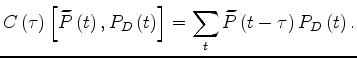
The cross-correlation
![]() between
the recorded data and the modeled data
is defined as a function of the correlation time lag
between
the recorded data and the modeled data
is defined as a function of the correlation time lag ![]() as
as
I introduce an objective function
that maximizes the flatness of the correlation function
along the receiver axis for all values of the lag ![]() .
In particular, I aim to maximize local correlation flatness
after subdividing the receiver array
into local subarrays.
To extract the correlation for each subarray
centered at
.
In particular, I aim to maximize local correlation flatness
after subdividing the receiver array
into local subarrays.
To extract the correlation for each subarray
centered at
 ,
I apply a local beam-decomposition
operators
,
I apply a local beam-decomposition
operators
![]() .
Within in each subarray,
traces are defined by the local offset
.
Within in each subarray,
traces are defined by the local offset
![]() .
The dimensions of each
.
The dimensions of each
![]() are thus
are thus
![]() .
.
Given a background slowness ![]() we can compute the correlation
in equation 1.
In each subarray,
the correlation can be flattened
by the application of
we can compute the correlation
in equation 1.
In each subarray,
the correlation can be flattened
by the application of
![]() moveout operators
moveout operators
![]() ;
that is
;
that is
| (A-2) |
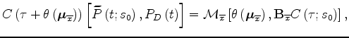 are the moveout parameters
and
are the moveout parameters
and I can now introduce the first, and local, term of the objective function that measures the flatness of the correlation within each subarray as:
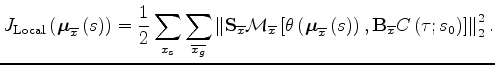 ,
but it depends indirectly from it through
the moveout parameters
.
These parameters are the solutions of
and
and the moved-out correlation computed with the background slowness
,
but it depends indirectly from it through
the moveout parameters
.
These parameters are the solutions of
and
and the moved-out correlation computed with the background slowness
For velocity estimation,
the most effective parametrization of the moveout within
each beam is the curvature ![]() ,
that defines the following moveout equation
,
that defines the following moveout equation
As the numerical examples I show in the next section demonstrate, the beam curvature is effective to capture the long-wavelength perturbations in the velocity model, but is less effective to capture the short-wavelength perturbations. Accordingly, a wave-equation tomography based solely on the objective function 3 may have difficulties to estimate short-wavelength velocity perturbations.
To address this shortcoming I introduce a second, and global, term to the objective function. This term measures flatness across the subarrays, after the local moveouts have been applied, and is defined as,
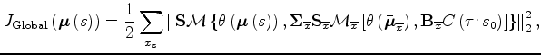 assembles all the results
of the stacking over the subarrays into a global array,
assembles all the results
of the stacking over the subarrays into a global array,
The global moveout parameters are the solutions of the following
![]() maximization problems
maximization problems
I chose to parametrize the global moveout
as simple time shifts for each beam center
![]() that is, the moveout equation is
that is, the moveout equation is
Combining the objective function in 3 and in 7 we define the maximization problem that we solve to estimate slowness:
|
|
|
|
Wave-equation tomography by beam focusing |