Wave-equation tomography by beam focusing

Numerical computation of search directions

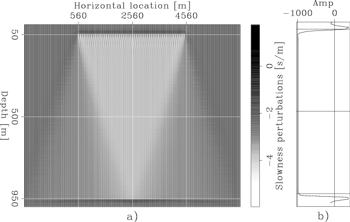
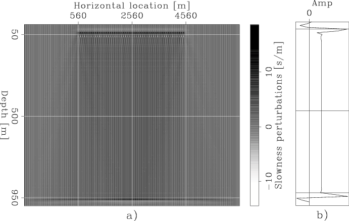
To test the method presented in the previous section, I computed the gradient of the objective functions for two synthetic data sets. The first assumes a uniform slowness error, whereas the second assumes a localized velocity error. In both cases the correct velocity was constant and equal to 1 km/s. Both sets of experiments were computed assuming 50 shots at the surface (actually at 50 meters depth) spaced 80 meters apart, and the receiver array at a depth of 950 meters. The data modeled with a uniform slowness error were recorded by a split-spread array of 512 receivers spaced 10 meters apart, whereas the data modeled with a localized velocity error were recorded by a split-spread array of 720 receivers spaced 10 meters apart. In both cases, the receiver array was moving along with the shots, to maintain a uniform offset coverage for each shot. For the sake of clarity, for all the cases the figures display the search directions instead of the gradients. Also notice that I am showing separately the search directions computed for each term of the proposed objective function, without showing their sum. At the moment of writing this report, I am not confident of the relative scaling between the gradient computed for the local objective function and the gradient computed for the global one.

Avg-Dir-tiny-neg Figure 1. Search direction computed using conventional full-waveform inversion with a positive small ($0.1 \%$ ) uniform slowness error: a) slowness perturbations and b) slowness perturbations averaged over the horizontal direction.

Avg-Dir-large-neg Figure 2. Search direction computed using conventional full-waveform inversion with a positive large ($8.0 \%$ ) uniform slowness error: a) slowness perturbations and b) slowness perturbations averaged over the horizontal direction.

Wave-equation tomography by beam focusing