Kinematics in iterated correlations of a passive acoustic experiment

Stationary phases in iterated correlations

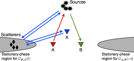
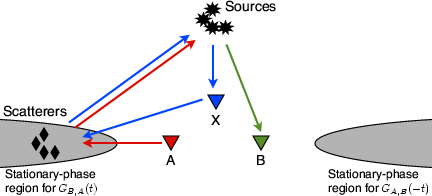
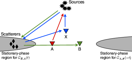
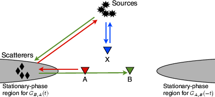
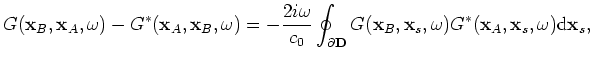
We proceed by studying the stationary phases of terms 15.6, 15.7, 15.10 and 15.11 in the iterated correlation. All terms correspond to particular combinations of ray paths.

Figure 5 shows for each term a graphical illustration of the combination of ray paths. Ray paths towards the source are subtracted from the ray paths emitting from the source, as in the correlation process (a convolution of one Green's function with the time reverse of another Green's function).

mainC4drawnew1,mainC4drawnew2,mainC4drawnew3,mainC4drawnew4
Figure 5. Geometrical interpretation of the correlations in terms 15.6, 15.7, 15.10 and 15.11 respectively in a) b) c) and d). $\mathbf{[NR]}$

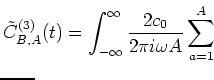
The time domain of equation 15, including only the terms of group 2, is given as

$$\tilde{C}^{(3)}_{B,A}(t) = \int_{-\infty}^{\infty} \frac{2c_0}{2\pi i\omega A } \displaystyle\sum_{a=1}^{A} \hspace{-4cm}$$ (40)

$$a_0(\mathbf{x}_B,\mathbf{x}_s,\omega)a_1^*(\mathbf{x}_{X,a},\math... ...1(\mathbf{x}_{X,a},\mathbf{x}_s,\omega) \mathrm{exp} \left\{ i\Omega_1 \right\} + \notag$$ (41)

$$a_0(\mathbf{x}_B,\mathbf{x}_s,\omega)a_1^*(\mathbf{x}_{X,a},\math... ...0(\mathbf{x}_{X,a},\mathbf{x}_s,\omega) \mathrm{exp} \left\{ i\Omega_2 \right\} + \notag$$ (42)

$$a_1(\mathbf{x}_B,\mathbf{x}_s,\omega)a_0^*(\mathbf{x}_{X,a},\math... ...1(\mathbf{x}_{X,a},\mathbf{x}_s,\omega) \mathrm{exp} \left\{ i\Omega_3 \right\} + \notag$$ (43)

$$a_1(\mathbf{x}_B,\mathbf{x}_s,\omega)a_0^*(\mathbf{x}_{X,a},\math... ...0(\mathbf{x}_{X,a},\mathbf{x}_s,\omega) \mathrm{exp} \left\{ i\Omega_4 \right\} \mathrm{d}\mathbf{x}_x \mathrm{d}\omega, \notag$$ (44)

where $a_0$ and $a_1$ are amplitude factors. The rapid phases, 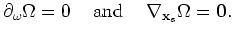$\Omega_1$, $\Omega_2$, $\Omega_3$ and $\Omega_4$ are found using equations A-6 and A-11; for a particular auxiliary station $\mathbf{x}_X$, we find

$$\Omega_1 \hspace{-.2cm}=\hspace{-.2cm} \omega \left[ t - c_0^{-1} \left\{ \vert\mathbf{x}_B - \mathbf{x}_s\vert - \vert\mathbf{x}_A - \mathbf{x}_s\vert \right\} \right], \hspace{.6cm}$$ (45)

$$\Omega_2 \hspace{-.2cm}=\hspace{-.2cm} \omega \left[ t - c_0^{-1} \left\{ \vert\mathbf{x}_B - \mathbf{x}... ..._c\vert + \vert\mathbf{x}_X - \mathbf{x}_s\vert \right\} \right], \hspace{.6cm}$$ (46)

$$\Omega_3 \hspace{-.2cm}=\hspace{-.2cm} \omega \left[ t - c_0^{-1} \left\{ \vert\mathbf{x}_B - \mathbf{x}... ..._s\vert + \vert\mathbf{x}_X - \mathbf{x}_c\vert \right\} \right], \hspace{.6cm}$$ (47)

$$\Omega_4 \hspace{-.2cm}=\hspace{-.2cm} \omega \left[ t - c_0^{-1} \left\{ \vert\mathbf{x}_B - \mathbf{x}_c\vert - \vert\mathbf{x}_A - \mathbf{x}_c\vert \right\} \right]. \hspace{.6cm}$$ (48)

We analyze these rapid phases using the stationary-phase method, keeping $\mathbf{x}_A$ and $\mathbf{x}_B$ fixed and varying $\mathbf{x}_X$, $\mathbf{x}_c$ and $\mathbf{x}_s$. According to the stationary-phase method, the dominant contribution to the integral and sum in equation 19 comes from positions of $\mathbf{x}_X$, $\mathbf{x}_c$ and $\mathbf{x}_s$ where

$$\partial_\omega \Omega=0, \hspace{1cm} \nabla_{\mathbf{x}_s} \Ome... ...pace{.5cm} \mathrm{and} \hspace{.5cm} \nabla_{\mathbf{x}_c} \Omega = \mathbf{0}$$ (49)

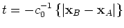
From the rapid phase, $\Omega_1$, of the first term in equation 19 we find stationary points for which

$$t=c_0^{-1} \left\{ \vert\mathbf{x}_B - \mathbf{x}_s\vert - \vert\mathbf{x}_A - \mathbf{x}_s\vert \right\}, \hspace{.5cm}$$ (50)

$$\nabla_{\mathbf{x}_s} \vert\mathbf{x}_B - \mathbf{x}_s\vert = \nabla_{\mathbf{x}_s} \vert\mathbf{x}_A - \mathbf{x}_s\vert ,$$ (51)

$$\nabla_{\mathbf{x}_X}\vert\mathbf{x}_B - \mathbf{x}_s\vert = \nabla_{\mathbf{x}_X} \vert\mathbf{x}_A - \mathbf{x}_s\vert,$$ (52)

$$\nabla_{\mathbf{x}_c} \vert\mathbf{x}_B - \mathbf{x}_s\vert = \nabla_{\mathbf{x}_c} \vert\mathbf{x}_A - \mathbf{x}_s\vert.$$ (53)

Conditions 27 and 28 are always satisfied. Condition 26 requires the stations to be on a line and the source to be on a line issuing from $\mathbf{x_s}$. When the stations and source are aligned as $\mathbf{x}_s \rightarrow \mathbf{x}_A \rightarrow \mathbf{x}_B$, condition 25 gives $t = c_0^{-1} \vert\mathbf{x}_B - \mathbf{x}_A\vert$. When the stations and source are aligned as $\mathbf{x}_s \rightarrow \mathbf{x}_B \rightarrow \mathbf{x}_A$, the first condition gives $t = - c_0^{-1}\vert\mathbf{x}_B - \mathbf{x}_A\vert$.

From the rapid phase, $\Omega_2$, of the first term in equation 19 we find stationary points for which

$$t =c_0^{-1} \left\{ \vert\mathbf{x}_B - \mathbf{x}_s\vert - \vert... ...thbf{x}_A - \mathbf{x}_c\vert + \vert\mathbf{x}_X - \mathbf{x}_s\vert \right\}, \hspace{.5cm}$$ (54)

$$\nabla_{\mathbf{x}_s} \left\{ \vert\mathbf{x}_B - \mathbf{x}_s\ve... ...thbf{x}_c - \mathbf{x}_s\vert - \vert\mathbf{x}_X - \mathbf{x}_s\vert \right\},$$ (55)

$$\nabla_{\mathbf{x}_X} \vert\mathbf{x}_X - \mathbf{x}_c\vert = \nabla_{\mathbf{x}_X} \vert\mathbf{x}_X - \mathbf{x}_s\vert,$$ (56)

$$-\nabla_{\mathbf{x}_c} \left\{ \vert\mathbf{x}_c - \mathbf{x}_s\v... ...thbf{x}_A - \mathbf{x}_c\vert + \vert\mathbf{x}_c - \mathbf{x}_s\vert \right\}.$$ (57)

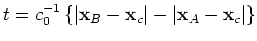
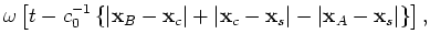
Condition 30 requires that station B, auxiliary station, the scatterer are on a line issuing from the source. Condition 31 requires that the auxiliary station and the scatterer are on a line issuing from the source. Condition 32 requires that station $A$, an auxiliary station and a scatterer are on a line issuing from the source. In short, stations $A$ and $B$, an auxiliary station, and the scatterer all align on a line issuing from the source. When these are aligned as $\mathbf{x_s} \rightarrow \mathbf{x}_c \rightarrow \mathbf{x}_X \rightarrow \mathbf{x}_A \rightarrow \mathbf{x}_B$, then $\vert\mathbf{x}_X-\mathbf{x}_s\vert = \vert\mathbf{x}_X - \mathbf{x}_c\vert + \vert\mathbf{x}_c - \mathbf{x}_s\vert$, $\vert\mathbf{x}_c - \mathbf{x}_s\vert + \vert\mathbf{x}_A - \mathbf{x}_c\vert = \vert\mathbf{x}_A-\mathbf{x}_s\vert$, and condition 29 gives $t = c_0^{-1} \vert\mathbf{x}_B - \mathbf{x}_A\vert$. When stations $A$ and $B$ are reversed, condition 29 gives $t = - c_0^{-1}\vert\mathbf{x}_B - \mathbf{x}_A\vert$.

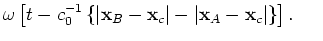
The rapid phase, $\Omega_3$, of the third term in equation 19 is similar to the rapid phase, $\Omega_2$, of the second term in equation 19. If stations $A$, $B$, an auxiliary station, and the scatterer are located on a line issuing from the source, aligned as $\mathbf{x_s} \rightarrow \mathbf{x}_c \rightarrow \mathbf{x}_X \rightarrow \mathbf{x}_A \rightarrow \mathbf{x}_B$, the dominant contribution resides at $t = c_0^{-1} \vert\mathbf{x}_B - \mathbf{x}_A\vert$. When stations $A$ and $B$ are interchanged, the dominant contribution of the third term in equation 19 resides at $t = - c_0^{-1}\vert\mathbf{x}_B - \mathbf{x}_A\vert$. Last we analyze the rapid phase, $\Omega_4$, of the fourth term in equation 19, and we find stationary points for which

$$t =c_0^{-1} \left\{ \vert\mathbf{x}_B - \mathbf{x}_c\vert - \vert\mathbf{x}_A - \mathbf{x}_c\vert \right\}, \hspace{.5cm}$$ (58)

$$\nabla_{\mathbf{x}_s} \vert\mathbf{x}_B - \mathbf{x}_c\vert = \nabla_{\mathbf{x}_s} \vert\mathbf{x}_A - \mathbf{x}_c\vert,$$ (59)

$$\nabla_{\mathbf{x}_X} \vert\mathbf{x}_B - \mathbf{x}_c\vert = \nabla_{\mathbf{x}_X} \vert\mathbf{x}_A - \mathbf{x}_c\vert,$$ (60)

$$\nabla_{\mathbf{x}_c} \vert\mathbf{x}_B - \mathbf{x}_c\vert = \nabla_{\mathbf{x}_c} \vert\mathbf{x}_A - \mathbf{x}_c\vert.$$ (61)

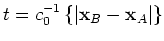
Conditions 34 and 35 are always satisfied. Condition 36 is satisfied when the scatterer lies on a line through stations $A$ and $B$. When stations $A$, $B$ and the scatterer are aligned as $\mathbf{x}_c \rightarrow \mathbf{x}_A \rightarrow \mathbf{x}_B$, condition 33 gives $t = c_0^{-1} \vert\mathbf{x}_B - \mathbf{x}_A\vert$. When stations $A$, $B$ and the scatterer align as $\mathbf{x}_c \rightarrow \mathbf{x}_B \rightarrow \mathbf{x}_A$, condition 33 gives $t = - c_0^{-1}\vert\mathbf{x}_B - \mathbf{x}_A\vert$.

Kinematics in iterated correlations of a passive acoustic experiment