Kinematics in iterated correlations of a passive acoustic experiment

Example of Green's function iterated correlation

We next study how forming $C^{(3)}_{B,A}$ of a wave field excited by a single source can improve the retrieved Green's function in the presence of an auxiliary scatterer. We study a geometry where the main stations are located $200$ m distant from each other (see Figure 6). We use 512 auxiliary stations located on a circle with radius $300$ m centered between the two main stations. The source is located at $s'$, with a distance of $800$ m from the center and at an angle of $\phi=3/4\pi$ radians. There is a scatterer positioned at a distance of $550$ m from the center at an angle of $\phi=\pi$ radians.

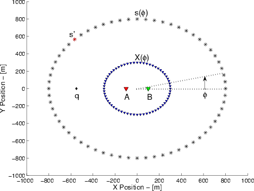
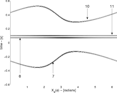
geomC4 Figure 6. Experiment geometry for the evaluation of $C^{(3)}_{B,A}$. $\mathbf{[ER]}$

We omit the terms of group 3 in equation 15, because their contribution is at least of order $\alpha$ weaker than those in group 2. $C^{(2)}$ is evaluated between stations $A$ or $B$ and all the auxiliary stations $X$, yielding $C^{(2)}_{A,X}$ and $C^{(2)}_{B,X}$; the obtained correlograms are shown in Figures 7(a) and 7(b). We evaluate $C^{(3)}_{B,A}$ for each auxiliary station, including all terms of groups 1 and 2, and compile the result in a correlogram shown in Figure 8(a).

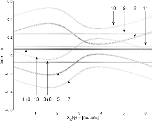
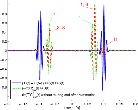
The contribution of each term is labeled according to the numbering of equation 15. We sum $C^{(3)}_{B,A}$ over the auxiliary stations, according to equation 18, to obtain the retrieved signal in Figure 8(b). We compare this signal to the true result, convolved with the square of the autocorrelation of the wavelet $S(\omega)$, and the result retrieved by correlating stations $B$ and $A$ directly ( $C^{(2)}_{B,A}$) weighted by $-i\omega S(\omega)$. It is clear that the dominant contribution in $C^{(3)}_{B,A}$, without muting $C^{(2)}_{A,X}$ and $C^{(2)}_{B,X}$, does not correspond to the direct event between the stations $A$ and $B$. If we assume we can perfectly mute only the dominant term 4.1 from $C^{(2)}_{A,X}$ and $C^{(2)}_{B,X}$, this would leave the terms of group 2.

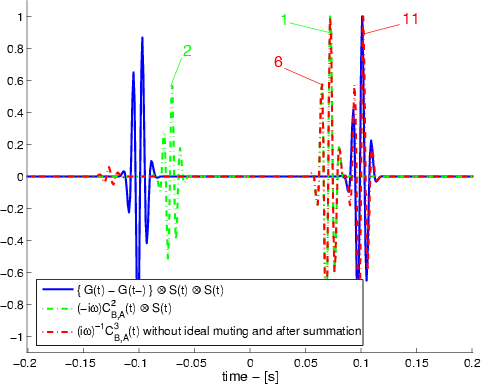
A correlogram of their contributions to $C^{(3)}_{B,A}$ is shown in Figure 9(a), summing this panel and multiplying with a phase-modifying according to equation 18, leads to the signal in Figure 9(b). We now see that there is a dominant term coinciding with the causal direct event between stations $A$ and $B$ in the true result; this event comes from term 15.11.

corrC2a,corrC2b
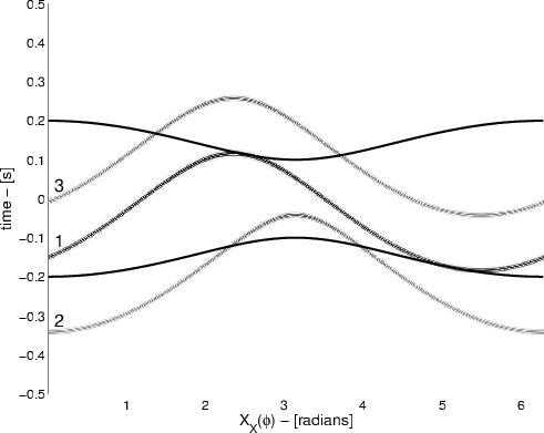
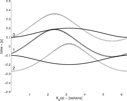
Figure 7. a) Correlogram for correlations between station $A$ and all auxiliary stations as a function of auxiliary station-position angle. Black lines indicates traveltime of a wave from station $A$ to each auxiliary station. b) Correlogram for correlations between station $B$ and all auxiliary stations as a function of auxiliary station-position angle. Black line indicates traveltime of a wave from station or $B$ to each auxiliary station. $\mathbf{[ER]}$

corrC4ABa,resultC4a
Figure 8. a) Correlogram of $C^{(3)}_{B,A}$ for each auxiliary station, including all 11 terms in groups 1 and 2 of equation 15. b) Correlogram of $C^{(3)}_{B,A}$ for each auxiliary station, including only the 4 terms from groups 2 of equation 15. $\mathbf{[ER]}$

corrC4ABb,resultC4b
Figure 9. a) Comparison of reconstructed Green's function with the true result, after summation of all 11 terms of groups 1 and 2 over auxiliary station. b) Comparison of reconstructed Green's function with true result, after summation of 4 terms of group 2 over auxiliary station. $\mathbf{[ER]}$

Kinematics in iterated correlations of a passive acoustic experiment