Kinematics in iterated correlations of a passive acoustic experiment

Green's function retrieval by iterated correlations

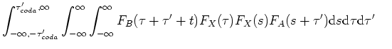
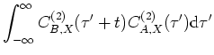
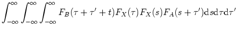
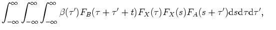
In the absence of complete source coverage, we can make use of the scattering properties of the medium to mitigate the directivity of the wave field. The iterated correlation between stations $B$ and $A$ is defined using auxiliary station X as follows:

$$C^{(3)}_{B,A}(t) = \int_{-\infty}^{\infty}C^{(2)}_{B,X}(\tau'+t)C^{(2)}_{A,X}(\tau')\mathrm{d}\tau'\notag$$ (18)

$$= \int_{-\infty}^{\infty} \int_{-\infty}^{\infty} \int_{-\infty}^{\... ...\tau) F_{X}(s) F_{A}(s+\tau') \mathrm{d}s \mathrm{d}\tau \mathrm{d}\tau' \notag$$ (19)

$$= \frac{1}{2\pi}\int_{-\infty}^{\infty} F_{B}(\omega)F^*_{X}(\omega... ...}(\omega)F_{A}^*(\omega) \mathrm{exp}\left\{ i\omega t\right\}\mathrm{d}\omega$$ (20)

The Green's function in the Born approximation for a scattering medium is composed of two terms; $C^{(3)}_{B,A}$ therefore contains $2^4=16$ terms

$$C^{(3)}_{B,A} = G_0(\mathbf{x}_B,\ma... ...mathbf{x}_X,\mathbf{x}_{s},\omega) + \hspace{.5cm}(\ref{eq:C4}.1) \hspace{.2cm}$$ (21)

$$G_0(\mathbf{x}_B,\mathbf{x}_{s},\ome... ...}_X,\mathbf{x}_{s},\omega) + \hspace{.5cm} (\ref{eq:C4}.2) \hspace{.2cm} \notag$$ (22)

$$G_0(\mathbf{x}_B,\mathbf{x}_{s},\ome... ...}_X,\mathbf{x}_{s},\omega) + \hspace{.5cm} (\ref{eq:C4}.3) \hspace{.2cm} \notag$$ (23)

$$G_0(\mathbf{x}_B,\mathbf{x}_{s},\ome... ...}_X,\mathbf{x}_{s},\omega) + \hspace{.5cm} (\ref{eq:C4}.4) \hspace{.2cm} \notag$$ (24)

$$G_0(\mathbf{x}_B,\mathbf{x}_{s},\ome... ...}_X,\mathbf{x}_{s},\omega) + \hspace{.5cm} (\ref{eq:C4}.5) \hspace{.2cm} \notag$$ (25)

$$G_0(\mathbf{x}_B,\mathbf{x}_{s},\ome... ...}_X,\mathbf{x}_{s},\omega) + \hspace{.5cm} (\ref{eq:C4}.6) \hspace{.2cm} \notag$$ (26)

$$G_0(\mathbf{x}_B,\mathbf{x}_{s},\ome... ...}_X,\mathbf{x}_{s},\omega) + \hspace{.5cm} (\ref{eq:C4}.7) \hspace{.2cm} \notag$$ (27)

$$G_0(\mathbf{x}_B,\mathbf{x}_{s},\ome... ...}_X,\mathbf{x}_{s},\omega) + \hspace{.5cm} (\ref{eq:C4}.8) \hspace{.2cm} \notag$$ (28)

$$G_1(\mathbf{x}_B,\mathbf{x}_{s},\ome... ...}_X,\mathbf{x}_{s},\omega) + \hspace{.5cm} (\ref{eq:C4}.9) \hspace{.2cm} \notag$$ (29)

$$G_1(\mathbf{x}_B,\mathbf{x}_{s},\ome... ...G_1(\mathbf{x}_X,\mathbf{x}_{s},\omega) + \hspace{.5cm} (\ref{eq:C4}.10) \notag$$ (30)

$$G_1(\mathbf{x}_B,\mathbf{x}_{s},\ome... ...G_0(\mathbf{x}_X,\mathbf{x}_{s},\omega) + \hspace{.5cm} (\ref{eq:C4}.11) \notag$$ (31)

$$G_1(\mathbf{x}_B,\mathbf{x}_{s},\ome... ...G_1(\mathbf{x}_X,\mathbf{x}_{s},\omega) + \hspace{.5cm} (\ref{eq:C4}.12) \notag$$ (32)

$$G_1(\mathbf{x}_B,\mathbf{x}_{s},\ome... ...G_0(\mathbf{x}_X,\mathbf{x}_{s},\omega) + \hspace{.5cm} (\ref{eq:C4}.13) \notag$$ (33)

$$G_1(\mathbf{x}_B,\mathbf{x}_{s},\ome... ...G_1(\mathbf{x}_X,\mathbf{x}_{s},\omega) + \hspace{.5cm} (\ref{eq:C4}.14) \notag$$ (34)

$$G_1(\mathbf{x}_B,\mathbf{x}_{s},\ome... ...G_0(\mathbf{x}_X,\mathbf{x}_{s},\omega) + \hspace{.5cm} (\ref{eq:C4}.15) \notag$$ (35)

$$G_1(\mathbf{x}_B,\mathbf{x}_{s},\ome... ...)G_1(\mathbf{x}_X,\mathbf{x}_{s},\omega). \hspace{.9cm} (\ref{eq:C4}.16) \notag$$ (36)

Three groups of terms can be distinguished; group 1 includes terms 15.1, 15.2, 15.3, 15.4, 15.5, 15.9 and 15.13, which are terms correlating with the dominant contribution in $C^{(2)}$; $G_0G_0^*$. Group 2 contains the terms of interest in this paper; 15.6, 15.7, 15.10 and 15.11; see the stationary-phase analysis below. The third group contains events that are of order $\alpha^3$ and includes terms 15.8, 15.12, 15.14, 15.15 and 15.16. The leading term in $C^{(2)}$ contributes to a spurious term, because the source is not located at a stationary angle of the event between stations A and B. To exclude the terms of group 1, we remove the dominant term after forming $C^{(2)}_{B,X}$ and $C^{(2)}_{A,X}$. This is done by muting the correlation in the time domain to suppress all times smaller than $\tau_{coda}$:

$$C^{(3)}_{B,A}(t) = \int_{-\infty,-\tau'_{coda}}^{\tau'_{coda},\infty} \int_{-\infty}... ..._{X}(s) F_{A}(s+\tau') \mathrm{d}s \mathrm{d}\tau \mathrm{d}\tau' \hspace{.5cm}$$ (37)

$$= \int_{-\infty}^{\infty} \int_{-\infty}^{\infty} \int_{-\infty}^{\... ...{X}(s) F_{A}(s+\tau') \mathrm{d}s \mathrm{d}\tau \mathrm{d}\tau', \hspace{.5cm}$$ (38)

where $\tau_{coda}$ is defined as an estimated traveltime between the main stations and the auxiliary stations, $\beta(\tau)$ is a muting function that is zero for $\beta(\tau)=0 \mathrm{for} \tau : [-\tau_{coda} : \tau_{coda}]$ and otherwise $\beta(\tau)=1$.

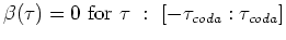We learned from Figure 3 that the dominant term always arrives within that time window. We average the iterated correlations over a network of $A$ auxiliary stations and include a phase-modifying term,

$$\tilde{C}^{(3)}_{B,A}(\omega) = \frac{2c_0}{i\omega A} \displaystyle\sum_{a=1}^{A} C^{(3)}_{B,A}(\omega),$$ (39)

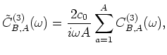where $\tilde{C}^{(3)}_{B,A}(\omega)$ is an implicit function of auxiliary-station position $\mathbf{x}_{X,a}$, according to equation 15. The phase-modifying proportionality factor is chosen such that the $\frac{\omega^2}{c_0^2}$ factor in the Born approximation (see equation A-10) is matched to the $\frac{-2i\omega}{c_0}$ factor in conventional interferometry (equation 2).

Kinematics in iterated correlations of a passive acoustic experiment