Kinematics in iterated correlations of a passive acoustic experiment

Frequency-domain Green's function in homogeneous media

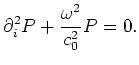
Using the forward Fourier transformation equation A-2, the wave equation for pressure in a homogeneous medium with $c(\mathbf{x})=c_0$ is written in the frequency-domain as

$$\partial^2_i P + \frac{\omega^2}{c_0^2} P = 0.$$ (65)

The frequency-domain Green's function $G = G(\mathbf{x},\mathbf{x}_s,\omega)$ is defined by introducing an impulsive point source acting at 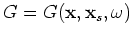$t=0$ and $\mathbf{x}=\mathbf{x}_s$ on the right-hand side of equation A-4 as follows:

$$\partial^2_{i} G + \frac{\omega^2}{c_0^2} G = -\delta(\mathbf{x}-\mathbf{x}_s).$$ (66)

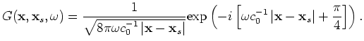
The Green's function solution for two-dimensional space, under the far field approximation can be obtained as

$$G(\mathbf{x},\mathbf{x}_s,\omega) = \frac{1}{\sqrt{8\pi\omega c_0... ...\left\vert \mathbf{x}-\mathbf{x}_s \right\vert + \frac{\pi}{4} \right] \right).$$ (67)

A source function is easily included by multiplication with the frequency-domain source function. A measurement, $P_A(\omega)$, at a station located at $\mathbf{x}_A$ of a source at $\mathbf{x}_s$ emitting a source function $s(\omega)$ is obtained as follows:

$$P_A = G(\mathbf{x}_A,\mathbf{x}_s,\omega)s(\omega).$$ (68)

The sources in this paper are simulated emitting zero-phase Ricker wavelets with center frequency $\omega_0$. The frequency-domain expression used is

$$s(\omega) = \frac{2 \omega^2}{\sqrt{\pi} \omega_0^3} \mathrm{exp}\left( -\frac{\omega^2}{\omega_0^2} \right).$$ (69)

Kinematics in iterated correlations of a passive acoustic experiment