|
|
|
|
Joint wave-equation inversion of time-lapse seismic data |
The computational cost of the full Hessian matrix for one survey (needless to say for multiple surveys) is prohibitive and not practical for any reasonably sized survey.
Several authors have discussed possible approximations to the wave-equation Hessian (Symes, 2008; Guitton, 2004; Tang, 2008a; Shin et al., 2001; Rickett, 2003; Valenciano, 2008; Tang, 2008b) .
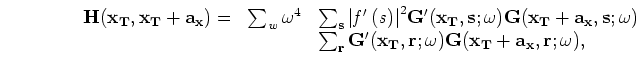
The wave-equation Hessian for synthetic seismic data,
![]() at a given frequency,
at a given frequency,
![]() , recorded by receiver
, recorded by receiver
![]() , from a shot
, from a shot
![]() and scattering point
and scattering point
![]() , is given by
, is given by
 corresponds to all model points. A detailed derivation of the explicit wave-equation Hessian is given by Mulder and Plessix (2004).
Because reservoirs are typically limited in extent, the region of interest is usually smaller than the full image space. Thus, the required Hessian matrices are constructed for a region around the target zone and not for the full survey area. In this paper, we follow the target-oriented approach of Valenciano (2008) in the Hessian computation. Phase-encoding approximations to the target-oriented Hessian (Tang, 2008a) offer improved efficiency in the Hessian computation and are currently being explored as alternatives to the explicit method used in this paper.
The target oriented Hessian (Valenciano, 2008) is given by:
where
 is the offset from the target image-point
![]() defining the filter size and hence the number of off-diagonal terms to be computed.
The filter size
can be determined heuristically or from an analysis of the amplitudes of filter coefficients away from the diagonal.
As noted by Valenciano (2008), the frequency sampling required to prevent wrap-around artifacts for the local filter (or row of the Hessian) for a given image point is coarser than that used in migration.
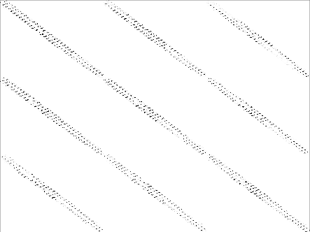
Examples of the target-oriented Hessian operator for the model in Figures 1 and three surveys are shown in Figures 2 and 3 for both RJID and RJMI.
defining the filter size and hence the number of off-diagonal terms to be computed.
The filter size
can be determined heuristically or from an analysis of the amplitudes of filter coefficients away from the diagonal.
As noted by Valenciano (2008), the frequency sampling required to prevent wrap-around artifacts for the local filter (or row of the Hessian) for a given image point is coarser than that used in migration.
Examples of the target-oriented Hessian operator for the model in Figures 1 and three surveys are shown in Figures 2 and 3 for both RJID and RJMI.

|
|---|
|
surv5-salt-imp
Figure 1. Full impedance model. The box indicates the target area for which Figures 2 and 3 were computed, while the anomaly centered at distance 0m and depth |
|
|
|
hesssalt3
Figure 2. JID: Joint target-oriented Hessian operator for one baseline and two monitor surveys for the reservoir models in Figure 1. The dimension of the square matrix here and in Figure 3 is equal to the number of surveys times the size of the model space. This figure corresponds to the |
|
|---|---|
|
|
|
hesssaltjimi3
Figure 3. JMI: Joint target-oriented Hessian for one baseline and two monitor surveys for the reservoir models in Figure 1. See caption in Figure 2 for further description. [NR] |

|
|---|---|
|
|
In a single survey, each row of the Hessian is a point-spread function that describes the effects of the limited-bandwidth seismic waveform, geometry and illumination on a reflectivity spike in the subsurface. In multiple surveys, each band belonging to individual sub-matrices contains similar information from a single or combination of surveys as shown in equations A-25 and A-12. In addition, note that the empty bins in Figures 2 and 3 are neither computed nor stored and that because of the matrix symmetry, only one-half of its elements needs to be computed. The structure of the problem gives a large leeway for parallelization over several domains in both the Hessian computation and inversion. Finally, since we assume that there is not a significant variation in the background velocity between surveys, and since some shot and receiver locations would be re-occupied during the monitor survey(s), some Green's functions can be reused in the Hessian computation for different surveys.
|
|
|
|
Joint wave-equation inversion of time-lapse seismic data |