 |
 |
 |
 | Joint wave-equation inversion of time-lapse seismic data |  |
![[pdf]](icons/pdf.png) |
Next: Discussion
Up: Ayeni and Biondi: Joint
Previous: Target-oriented Hessian
The inversion formulations were tested on synthetic datasets modeled for the 2D-synthetic sub-salt model in Figure 1.
We simulated six datasets (representing different stages of production) using a variable-density acoustic finite-difference algorithm.
Reservoir changes were modeled as an expanding Gaussian anomaly centered at x = 0m and z =  m.
In order to simulate non-repeated acquisition geometries, we modeled all the datasets with spatially different geometries as summarized in Table 1.
We modeled
m.
In order to simulate non-repeated acquisition geometries, we modeled all the datasets with spatially different geometries as summarized in Table 1.
We modeled  shots spaced at
  m and
m and  receivers spaced at
  m and for each survey, the receiver spread was kept constant while the shots move along.
We consider that reflectivity change is most influenced by a change in the density within the reservoir and that there is not a significant change in the background velocity model between surveys.
The spatial regularization operator is a gradient along reflector dips, while a temporal gradient was used to ensure temporal smoothness.
m and for each survey, the receiver spread was kept constant while the shots move along.
We consider that reflectivity change is most influenced by a change in the density within the reservoir and that there is not a significant change in the background velocity model between surveys.
The spatial regularization operator is a gradient along reflector dips, while a temporal gradient was used to ensure temporal smoothness.
Table 1:
Modeling parameters for synthetic datasets
| |
Shot/receiver depth |
Shot/receiver spread |
| Geometry 1 |
0m |
 to m to m |
| Geometry 2 |
 m m |
 to to  m m |
| Geometry 3 |
 m m |
 to to  m m |
| Geometry 4 |
 m m |
 to to  m m |
| Geometry 5 |
 m m |
 to to  m m |
| Geometry 6 |
 m m |
 to to  m m |
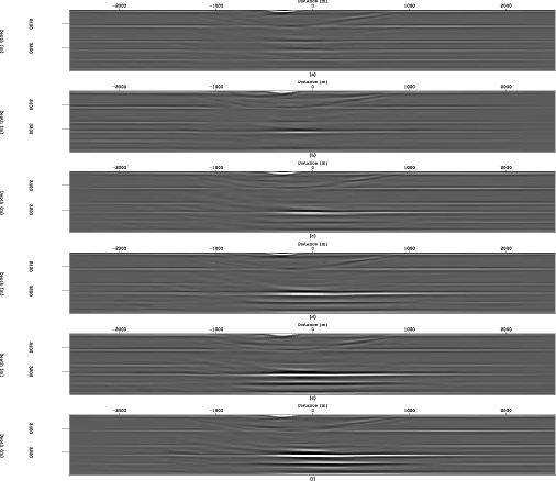
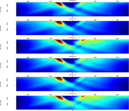
Figure 4 shows the migrated images for the six surveys, while corresponding illumination maps (diagonal of the Hessian) are shown in Figure 5.
The irregular illumination patterns explain the uneven amplitudes of reflectors below the salt in Figure 4.
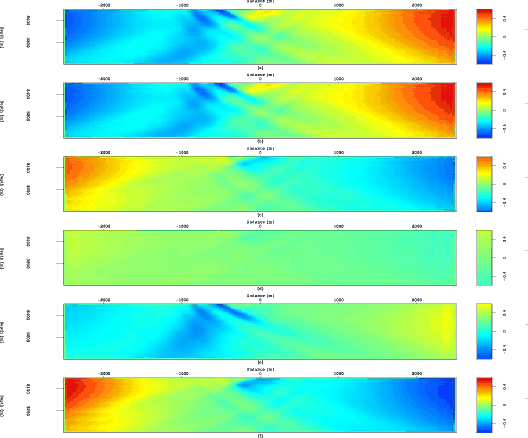
Figure 6 shows the illumination-ratio (normalized rms-difference in illumination) between baseline and the monitor surveys, which measures of the variability of illumination between surveys.
We represent the variation in illumination at any image point as the illumination-ratio between the point-spread functions for the different surveys.
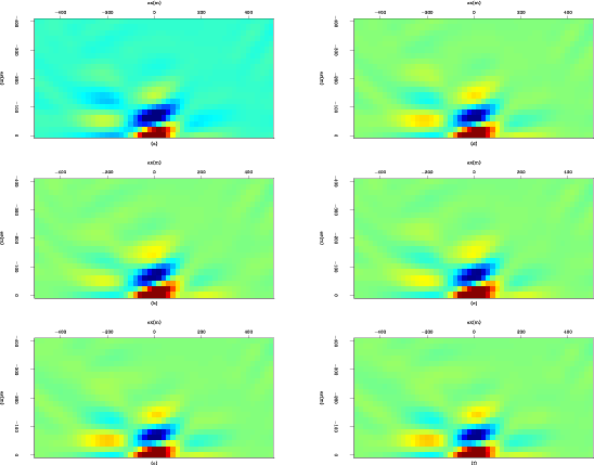
For example, Figure 7 shows the point-spread functions at image point
![$ [x=-200m, z=2800m]$](img9.png) ,
while Figure 8 shows the coresponging illumination-ratio.
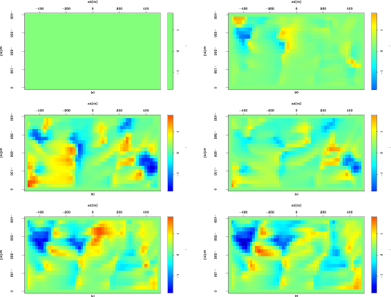
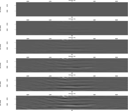
The time-evolution of the true reflectivity model is shown in Figure 9 and the inversion goal is to reconstruct these.
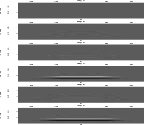
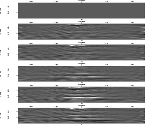
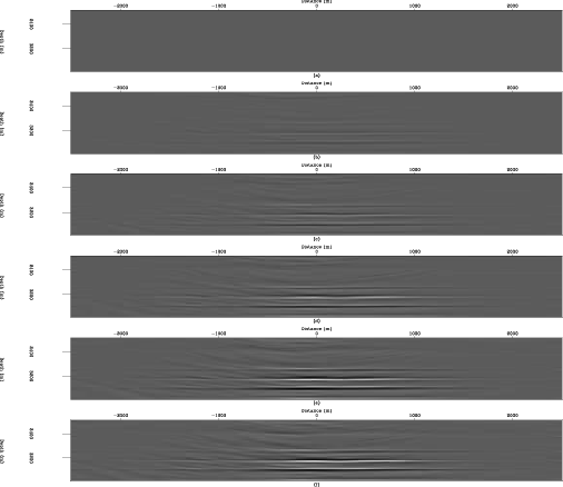
Figure 10 is the reflectivity change obtained from migration, while Figures 11 to 13 were obtained from separate inversion, RJID and RJMI respectively.
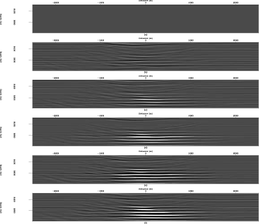
Both the RJID and RJMI results contain less noise relative to migration (Figures 10) and separate inversion (Figures 11).
No pre-processing was done to remove multiples from the data and hence these are expected to adversely affect the inversion.
,
while Figure 8 shows the coresponging illumination-ratio.
The time-evolution of the true reflectivity model is shown in Figure 9 and the inversion goal is to reconstruct these.
Figure 10 is the reflectivity change obtained from migration, while Figures 11 to 13 were obtained from separate inversion, RJID and RJMI respectively.
Both the RJID and RJMI results contain less noise relative to migration (Figures 10) and separate inversion (Figures 11).
No pre-processing was done to remove multiples from the data and hence these are expected to adversely affect the inversion.
|
|---|
migs
Figure 4. Migrated images obtained for six surveys (see modeling parameters in Table 1) for the target area in shown Figure 1.
Figure (a) is the baseline image, while Figures (b)-(f) are images of the monitor images.
Note the irregular amplitude patterns cause by the presence of the overlying salt structure.[CR]
|
|---|
![[png]](icons/viewmag.png)
|
|---|
|
|---|
illums-salt
Figure 5. Illumination maps for the six surveys described in Table 1.
Each section corresponds to the migrated sections in Figure 4 and explain the observed irregular seismic amplitudes. Light color represent high illumination and dark represents low illumination.[CR]
|
|---|
|
|
|---|
|
|---|
illums-salt-r
Figure 6. Base-Monitor illumination-ratio for the six surveys described in Table 1.
Each section corresponds to a normalized rms-ratio (over 3x3 patches) between the Hessian diagonal of the monitor surveys (Figure 5b-f) to that of the baseline (Figure 5a).[CR]
|
|---|
|
|
|---|
|
|---|
hess-salt-off
Figure 7. Point spread functions at the image point
for the six surveys in Figure 5.
Each section corresponds to a row of the Hessian for the images in Figure 4a-f).
Note that only one half of each filter is computed, since the Hessian matrix is symmetric.[CR]
|
|---|
|
|
|---|
|
|---|
illums-salt-off
Figure 8. Base-Monitor illumination-ratio at image point
for the six surveys described in Table 1.
section corresponds to a normalized rms-ratio (over 3x3 patches) between the point-spread functions (a row of the Hessian) of the monitor surveys (Figure 7b-f) to that of the baseline (Figure 7a).[CR]
|
|---|
|
|
|---|
|
|---|
refs4d
Figure 9. True cumulative time-lapse reflectivity images at the times for which the six surveys (Table 1) were modeled. These should be compared with the results in Figures 10 to 13.[CR]
|
|---|
|
|
|---|
|
|---|
migs4d
Figure 10. Migrated time-lapse at six different times corresponding to Figure 4. Each section shows the amplitude change between time 1 (baseline) and the time of the monitor survey.
Note that the inversion has resulted in an increase in the noise amplitudes relative to migrated time-lapse images shown in Figure 10.[CR]
|
|---|
|
|
|---|
|
|---|
invs4d
Figure 11. Separately inverted time-lapse images at six different times. Each section shows the amplitude change between time 1 (baseline) and the time of the monitor survey.
Note that the inversion has resulted in an increase in the noise amplitudes relative to migrated time-lapse images shown in Figure 10.[CR]
|
|---|
|
|
|---|
|
|---|
inv14d
Figure 12. RJID: Jointly inverted time-lapse images at six different times. Each section shows the amplitude change between time 1 (baseline) and the time of the monitor survey.
Compare these results to Figures 9, 10, 11 and 13.[CR]
|
|---|
|
|
|---|
|
|---|
inv24d
Figure 13. RJMI: Jointly inverted time-lapse images at six different times. Each section shows the amplitude change between time 1 (baseline) and the time of the monitor survey.
Compare these results to Figures 9, 10, 11 and 12.[CR]
|
|---|
|
|
|---|
|
|
|
|
| Joint wave-equation inversion of time-lapse seismic data | |
|
Next: Discussion
Up: Ayeni and Biondi: Joint
Previous: Target-oriented Hessian
2009-04-13