|
|
|
|
Joint wave-equation inversion of time-lapse seismic data |
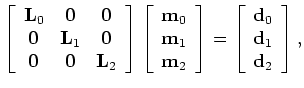 are respectively datasets for the baseline, first and second monitor,
 ,
respectively.
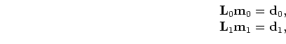
The least-squares solution to equation A-7 is given as
,
respectively.
The least-squares solution to equation A-7 is given as
We rewrite equation A-8 as
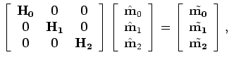 is the migrated image from the
 and
and
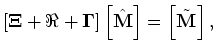
 |
(A-13) |
 is given as
|
|
|
|
Joint wave-equation inversion of time-lapse seismic data |
![$\displaystyle \left [ \begin{array}{ccc} {\bf L}_{0} & {\bf0} & {\bf0} {\bf0...
...gin{array}{ccc} {\bf d}_{0} {\bf d}_{1} {\bf d}_{2} \end{array} \right ],$](img118.png)
![$\displaystyle \left [ \begin{array}{ccc} {\bf H_0}&{\bf0}&{\bf0} {\bf0}&{\bf ...
...c} \tilde {\bf m_0} \tilde {\bf m_1} \tilde {\bf m_2} \end{array} \right ],$](img123.png)
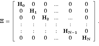
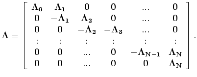
![$\displaystyle \left [ {\bf\Xi } + {\bf\Re } + {\bf\Gamma} \right ] \left [ \hat{{\bf M}} \right ] = \left [ \tilde {\bf M} \right ],$](img73.png)
![$\displaystyle {\bf\Xi }= \left [ \begin{array}{cccccc} {\bf H_0}&{\bf0}&{\bf0}&...
...&{\bf0} {\bf0}&{\bf0}&{\bf0}&{\bf ...}&{\bf0}&{\bf H_N} \end{array} \right ].$](img128.png)
![$\displaystyle {\bf R }= \left [ \begin{array}{cccccc} {\bf R_{0}}&{\bf0}&{\bf0}...
...}&{\bf0} {\bf0}&{\bf0}&{\bf0}&{\bf0}&{\bf0}&{\bf R_N} \end{array} \right ],$](img130.png)
![$\displaystyle {\bf\Lambda }= \left [ \begin{array}{cccccc} {\bf\Lambda_{0}}&{\b...
...\bf0 }&{\bf0 }&{\bf ...}&{\bf0 }&{\bf0 }&{\bf\Lambda_{N}} \end{array} \right ].$](img131.png)
![$\displaystyle \hat{{\bf M}} = \left [ \begin{array}{cc} \hat{\bf m}_{0} \hat...
...{2} {\bf :} \hat{\bf m}_{N-1} \hat{\bf m}_{N} \end{array} \right ].$](img134.png)