Joint wave-equation inversion of time-lapse seismic data

Joint-inversion with Regularization

In most seismic monitoring problems, the general geology and reservoir architecture of the study area are known -- thus providing some information that can be used to determine appropriate regularization for the inversion. Such regularization incorporates prior knowledge of the reservoir geometry and location, and expectation of changes in different parts of the study area. As shown in the Appendix, the regularized joint-inversion for image difference (RJID) for two surveys is given by

$$\left ( \left [ \begin{array}{ccc} {\bf H_0+H_1} & {\bf H_1} {... ...ilde {\bf m}_{0}+\tilde {\bf m}_{1} \tilde {\bf m}_{1} \end{array} \right ],$$ (A-18)

where

$$\begin{array}{ccc} {\bf R_{ij} = { {\epsilon_i R'}_i \epsilon... ...j} = {{ \zeta_i \Lambda'}_i \zeta_j \Lambda_j}}, \end{array}$$ (A-19)

while 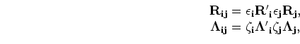${\bf R_0}$ and ${\bf R_1}$ are the spatial/imaging constraints for the baseline and time-lapse images respectively, and ${\bf {\Lambda}_0}$ and ${\bf {\Lambda}_1}$ the temporal regularization (or coupling) between the surveys. In the implementation of equation 19, the regularization terms, ${\bf {R}_{ij}}$ and ${\bf {\Lambda}_{ij}}$ are not explicitly computed, but instead, the appropriate operators ${\bf R_i}$ and ${\bf\Lambda_i}$ (and their adjoints, ${\bf R'_i}$ and ${\bf\Lambda'_i}$ respectively) are applied at each step of the inversion. The parameters ${\bf {\epsilon}_0}$ and ${\bf {\epsilon}_1}$ determine strength of the spatial regularization on the baseline and time-lapse images respectively, while ${\bf { \zeta }_0}$ and ${\bf {\zeta }_1}$ determine the coupling between surveys. The regularized joint-inversion of multiple images (RJMI) formulation for two surveys is given as

$$\left ( \left [ \begin{array}{ccc} {\bf H_0 } & {\bf0 } {\bf0 ... ...begin{array}{cc} \tilde {\bf m}_{0} \tilde {\bf m}_{1} \end{array} \right ].$$ (A-20)

The spatial regularization operator contains information on the structural geometry of the reservoir (or implied properties of correctly migrated gathers, e.g. horizontal angle gathers, or near-zero concentration of amplitudes in subsurface offset gathers), while the temporal regularization ensures that the reservoir changes evolve according to a reasonable scheme (e.g., smooth variation over time). The temporal regularization operator in the RJMI formulation is similar to that used in spatio-temporal tomographic inversion (Ajo-Franklin et al., 2005).

As shown in Appendix A, the general regularized joint-inversion problem can be written in compact notation as

$$\left [ {\bf\Xi } + {\bf\Re } + {\bf\Gamma} \right ] \left [ \hat{{\bf M}} \right ] = \left [ \tilde {\bf M} \right ],$$ (A-21)

where ${\bf\Xi }$ is the Hessian operator, 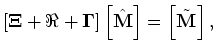${\bf\Re}$ is the spatial/imaging regularization operator, ${\bf\Gamma}$ is the temporal regularization operator, $\hat{\bf M}$ is the model vector and $\tilde {\bf M}$ the data vector. Each of the components of the RJID and RJMI formulations are fully described in Appendix A.

Note that in the RJID formulation, the imaging (baseline inversion) and monitoring (time-lapse inversion) goals are decoupled, thus allowing for application of different regularization schemes. Since the baseline and time-lapse images are expected to have different desirable properties, the baseline (${\bf R_0}$ and ${\bf\Lambda_0}$) and monitor (${\bf R_1}$ to ${\bf R_N}$ and ${\bf\Lambda_0}$ to ${\bf\Lambda_N}$) regularization operators are different. The RJMI formulation is cheaper to solve, since the joint Hessian operator is less dense and with appropriate regularization, the results from the two formulations should be comparable.

Joint wave-equation inversion of time-lapse seismic data