|
|
|
|
Joint wave-equation inversion of time-lapse seismic data |
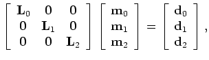 are respectively datasets for the baseline, first and second monitor,
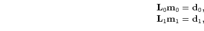 is the baseline reflectivity and the time-lapse reflectivities
 and
were acquired (with survey geometries defined by the linear
and
were acquired (with survey geometries defined by the linear
The least-squares solution to equation A-18 is given as
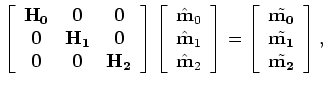 is the migrated image from the
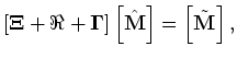
 is the temporal regularization between the surveys.
Note that
is the temporal regularization between the surveys.
Note that
 and
and
 |
(A-26) |
 is given as
 may be set to zero, since it is assumed that the original geological structure is unchanged over time or that geomechanical changes are accounted for before/during inversion.
|
|
|
|
Joint wave-equation inversion of time-lapse seismic data |
![$\displaystyle \left [ \begin{array}{ccc} {\bf L}_{0} & {\bf0} & {\bf0} {\bf ...
...gin{array}{ccc} {\bf d}_{0} {\bf d}_{1} {\bf d}_{2} \end{array} \right ],$](img135.png)
![$\displaystyle \left [ \begin{array}{ccc} {\bf {L'}_0 L_0+{L'}_1 L_1+{L'}_2 L_2}...
...begin{array}{c} {\bf d}_{0} {\bf d}_{1} {\bf d}_{2} \end{array} \right ],$](img139.png)
![$\displaystyle \left [ \begin{array}{ccc} {\bf H_0+H_1+H_2}&{\bf H_1+H_2}&{\bf H...
... \tilde {\bf m_1} + \tilde {\bf m_2} \tilde {\bf m_2} \end{array} \right ],$](img140.png)
![\begin{displaymath}\begin{array}{ll} \left ( \left [ \begin{array}{ccc} {\bf H_0...
... {\bf m_2} \tilde {\bf m_2} \end{array} \right ], \end{array}\end{displaymath}](img141.png)

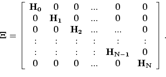
![$\displaystyle \left [ {\bf\Xi } + {\bf\Re } + {\bf\Gamma} \right ] \left [ \hat{{\bf M}} \right ] = \left [ \tilde {\bf M} \right ],$](img73.png)
![$\displaystyle {\bf R }= \left [ \begin{array}{cccccc} {\bf R_{0}}&{\bf0}&{\bf0}...
...}&{\bf0} {\bf0}&{\bf0}&{\bf0}&{\bf0}&{\bf0}&{\bf R_N} \end{array} \right ],$](img130.png)
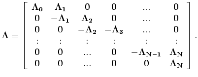
![$\displaystyle {\bf\Lambda }= \left [ \begin{array}{cccccc} {\bf\Lambda_{0}}&{\b...
...f0 }&{\bf0 }&{\bf ...}&{\bf0 }&{\bf0 }&{\bf\Lambda_{N}} \end{array} \right ].$](img149.png)
![$\displaystyle \tilde{{\bf M}} = \left [ \begin{array}{c} \tilde {\bf m_0}+{\bf ...
...{\bf m}_{N-1} + \tilde {\bf m}_{N} \tilde {\bf m}_{N} \end{array} \right ],$](img150.png)
![$\displaystyle \hat{{\bf M}} = \left [ \begin{array}{c} \hat{\bf m}_{0} \Delt...
...at{\bf m}_{2} { : } { : } \Delta \hat{\bf m}_{N} \end{array} \right ].$](img151.png)