ENHANCEMENTS OF THE METHOD: IRLS

A minor improvement in the method was the change from the Laplacian filter (3) in equation (2) to the gradient filter consisting of the two orthogonal first-order derivatives  

$${\bf A_1}= \begin{array} {\vert c\vert c\vert} \hline 1 & -1... ... {\vert c\vert} \hline 1 \ \hline -1 \ \hline\end{array}\,\,.$$ (4)

The reason for this change is evident in Figure 5. The gradient filter is more appropriate for the sharp edges (the first-derivative jump) of the lake bottom, while the Laplacian filter tends to smooth them out. This fact is related to the close correspondence between gradient filter smoothing and local linear interpolation on one side, and Laplacian smoothing and cubic (spline) interpolation on the other.

The major enhancement is the introduction of a weighting operator ${\bf W}$ into equation (1). Thus system (1) - (2) takes the form  

$${\bf 0 \approx W (d - Lm)}\;,$$ (5)

 

$${\bf 0 \approx \epsilon \, A_1 m}\;,$$ (6)

 

$${\bf 0 \approx \epsilon \, A_2 m}\;.$$ (7)

Though we didn't apply any formal straightforward theory to choose the weighting operator W, our heuristic choice followed two formal principles:

1.

Bad (inconsistent) data points are indicated by large values of the residual r = d - Lm left after conventional least squares inversion.

2.

Abnormally large residuals attract most of the conjugate gradient solver's efforts, directing it the wrong way. The residual should be whitened to distribute the solver's attention equally among all the data points and emphasize the role of the ``consistent majority.''

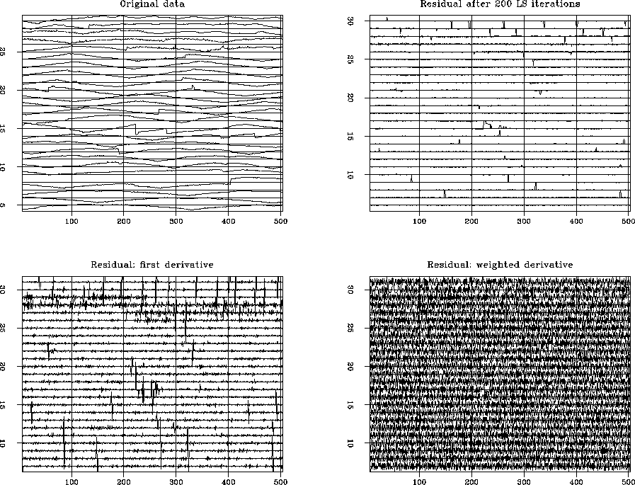
Figure 6 demonstrates changes in the residual space caused by the weighting. Each plot contains one long vector cut into several traces for better viewing. The top left plot is the original data from the patch used in the first experiments. The top right plot is the residual after 200 conventional conjugate gradient iterations. Note two major features of the residual distribution: statically shifted tracks (the zero-frequency component) and local bursts of energy (mostly in the upper part of the plot). To take away the zero-frequency component, we convolved the residual with the first-derivative operator. The result of differentiation appears on the bottom left plot. Finally, to take into account both large spikes created by differentiation and local bursts of energy, we constructed the following weighting function:  

$$w_i = w(r_i) = {{2\,\bar{r}} \over {\mid r_i \mid + \bar{r_i}}} \,.$$ (8)

Here $\bar{r}$ stands for the median of the absolute residual values from the whole data set, and $\bar{r_i}$ is the median in a small window around a current point r_i. The denominator of the weighting function is designed to reduce the value of the residual if it belongs either to a spike (large $\mid r_i \mid$) or to a local burst of energy (large $\bar{r_i}$). The numerator was chosen for scaling purposes. The bottom right plot in Figure 6 justifies our choice of the weighting function, displaying the residual derivative after weighting. The signal distribution resembles white noise in accordance with the second formal principle.

 

galdat
Figure 6 View from the data space (explanation in the text).

Thus the weighting operator ${\bf W}$ in equation (5) includes two components: the first-derivative filter ${\bf D}$ taken in the data space along the recording tracks and the weighting function w. Since w depends upon the residual, the inversion problem becomes nonlinear, and the algorithm approaches the IRLS class Scales et al. (1988).

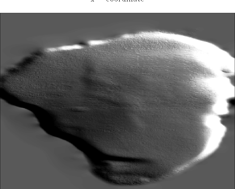
The result of the IRLS inversion is shown in Figure 7. While the noisy portions of the model disappeared as we had expected, a large-scale structure (valley) crossing the lake from north to south remained on the image. Comparison of Figures 9 and 10 demonstrates that the price for that improvement is a certain loss in the image resolution. This type of loss occurs because we rely on the model smoothing to remove the noise influence. The role of the smoothing increases when we apply IRLS in the manner of piece-wise linearization. The first step of the piece-wise linear algorithm is the conventional least squares minimization. The next step consists of reweighted least squares iterations made in several cycles with reweighting applied only at the beginning of each cycle. Thus the problem is linearized within a cycle, and the conjugate gradient solver opens each cycle with the steepest descent iteration. 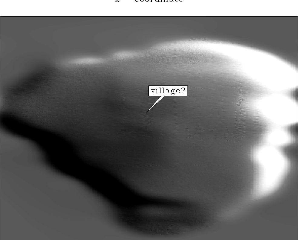What happens when the nonlinear reweighting is applied on each iteration is shown in Figure 8. Round ``villages'' on the bottom of the lake were identified as the consequence of occasional erroneous data points.

 

galrep
Figure 7 Result of the IRLS inverse interpolation (piece-wise linear).

 

galres
Figure 8 Result of the IRLS inverse interpolation (nonlinear).