

Next: TIME-FREQUENCY-STATISTICAL RESOLUTION
Up: Resolution
Previous: TIME-STATISTICAL RESOLUTION
Observations of sea level for a long period of time can be summarized in terms
of a few statistical averages
such as the mean height m and the variance  .Another important kind of statistical average for use on such
geophysical time series is the power spectrum.
Some mathematical
models explain only statistical averages of data and not the data themselves.
In order to recognize certain pitfalls and understand certain fundamental
limitations on work with power spectra,
we first consider an idealized example.
Let xt be a time series made up of independently chosen random numbers.
Suppose we have n of these numbers.
We can then define the data sample polynomial X(Z)
|  |
(38) |
We can now make up a power spectral estimate  from this sample of
random numbers by
|  |
(39) |
The difference between this and our earlier definition of spectrum is that
a power spectrum has the divisor n to keep the expected result from
increasing linearly with the somewhat arbitrary sample size n.
The definition of power spectrum is the expected value of  , namely
| ![\begin{displaymath}
R(Z) \eq E[\hat{R} (Z)]\end{displaymath}](img91.gif) |
(40) |
It might seem that a practical definition would be to let n tend to infinity
in (39).
Such a definition would lead us into a pitfall which is
the main topic of the present section.
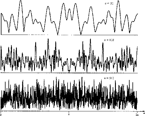
Specifically, from Figure 3 we conclude that  is a much fuzzier function than R(Z),
so that
|  |
(41) |
4-2
Figure 3 Amplitude spectra  of samples of n random numbers.
These functions seem to oscillate over about
the same range for n = 512 as they do for n = 32.
As n tends to infinity we expect infinitely rapid oscillation. of samples of n random numbers.
These functions seem to oscillate over about
the same range for n = 512 as they do for n = 32.
As n tends to infinity we expect infinitely rapid oscillation.
|
|  |

To understand why the spectrum is rough,
we identify coefficients of like powers of Z in (39).
We have
|  |
(42) |
enabling us
to write (39) for real time series  as
as
|  |
(43) |
Let us examine (43) for large n.
To do this,
we will need to know some of the statistical properties of the random numbers.
Let them have zero mean m = E(xt) = 0
and let them have known constant variance  and recall our assumption of independence which means that
E(xt xt+ s) = 0 if
  .Because of random fluctuations,
we have learned to expect that
  will come out to be
  plus
a random fluctuation component which decreases with sample size as
  ,namely
|  |
(44) |
Likewise,  should come out to be zero but the definition
(42) leads us to expect a fluctuation component
|  |
(45) |
For the kth correlation value k > 1 we expect a fluctuation of
order
|  |
(46) |
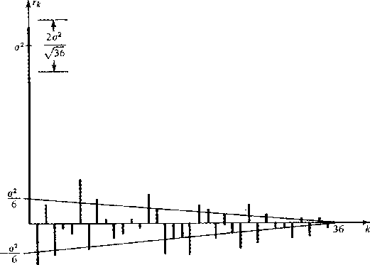
An autocorrelation of a particular set of random numbers is displayed in
Figure 4.
4-3
Figure 4 Positive lags
of autocorrelation of 36 random numbers.

Now one might imagine that as n goes to infinity the
fluctuation terms vanish and (39) takes the limiting form
 .Such a conclusion is false.
The reason is that although the
individual fluctuation terms go as
  the summation in
(43) contains n such terms.
Luckily, these terms are randomly
canceling one another so the sum does not diverge as
  .We recall
that the sum of n random signed numbers of unit magnitude is expected to
add up to a random number in the range
  .Thus the sum
(43) adds up to
|  |
(47) |
This is the basic result that a power spectrum estimated from the energy
density of a sample of random numbers has a fluctuation from frequency to
frequency and from sample to sample which is as large as the expected
spectrum.
It should be clear that letting n go to infinity does not take us to the
theoretical result  .The problem is that, as we increase n,
we increase the frequency resolution but not the statistical resolution.
To increase the statistical resolution we need to simulate ensemble averaging.
There are two ways to do this: (1) Take the
sample of n points and break it into k equal-length segments of n/k
points each.
Compute an
  for each segment and then add all k
of the
  together,
or (2) form
  from the n-point sample.
Of the n/2 independent amplitudes,
replace each one by an average over its k nearest neighbors.
Whichever method, (1) or (2),
is used it
will be found that
  and
and  inverse
of number of degrees of freedom averaged over = 1/k.
Thus, we have

If some of the data are not used,
or are not used effectively, we get the usual inequality

Thus we see that,
if there are enough data available (n large enough),
we can get as good resolution as we like.
Otherwise, improved statistical resolution
is at the cost of frequency resolution and vice versa.
We are right on the verge of recognizing a resolution tradeoff,
not only between  and
and  but also with
  ,the time duration of the data sample.
Recognizing now that the time duration of
our data sample is given by
  ,we obtain the inequality
|  |
(48) |
The inequality will be further interpreted and rederived from a somewhat
different point of view in the next section.
In time-series analysis we have the concept of coherency which is analogous
to the concept of correlation defined in Sec. 4-2.
There we had for two random variables x and y that
![\begin{displaymath}
c \eq {E(xy) \over [E(x^2)\, E(y^2)]^{1/2} }\end{displaymath}](img68.gif)
Now if xt and yt are time series,
they may have a relationship
between them which depends on time-delay, scaling, or even filtering.
For example, perhaps Y(Z) = F(Z) X(Z) + N(Z) where F(Z) is a filter and
nt is unrelated noise.
The generalization of the correlation concept is to define coherency by
![\begin{displaymath}
C \eq {E\left[ X \left( {1 \over Z}\right) \, Y(Z) \right] \over
[E(\overline {X} X)\, E(\overline {Y} Y)]^{1/2} }\end{displaymath}](img114.gif)
Correlation is a real scalar.
Coherency is complex and expresses the frequency dependence of correlation.
In forming an estimate of coherency it is
always essential to simulate some ensemble averaging.
Note that if the ensemble averaging were to be omitted,
the coherency (squared) calculation would give

which states that the coherency squared is +1 independent of the data.
Because correlation scatters away from zero we find that coherency squared is
biased away from zero.
4-4
Figure 5 Model of random time series generation.
|
|  |


Next: TIME-FREQUENCY-STATISTICAL RESOLUTION
Up: Resolution
Previous: TIME-STATISTICAL RESOLUTION
Stanford Exploration Project
10/30/1997
![]() , namely
, namely


![]() as
as


![]() .Such a conclusion is false.
The reason is that although the
individual fluctuation terms go as
.Such a conclusion is false.
The reason is that although the
individual fluctuation terms go as ![]() the summation in
(43) contains n such terms.
Luckily, these terms are randomly
canceling one another so the sum does not diverge as
the summation in
(43) contains n such terms.
Luckily, these terms are randomly
canceling one another so the sum does not diverge as ![]() .We recall
that the sum of n random signed numbers of unit magnitude is expected to
add up to a random number in the range
.We recall
that the sum of n random signed numbers of unit magnitude is expected to
add up to a random number in the range ![]() .Thus the sum
(43) adds up to
.Thus the sum
(43) adds up to
![]() .The problem is that, as we increase n,
we increase the frequency resolution but not the statistical resolution.
To increase the statistical resolution we need to simulate ensemble averaging.
There are two ways to do this: (1) Take the
sample of n points and break it into k equal-length segments of n/k
points each.
Compute an
.The problem is that, as we increase n,
we increase the frequency resolution but not the statistical resolution.
To increase the statistical resolution we need to simulate ensemble averaging.
There are two ways to do this: (1) Take the
sample of n points and break it into k equal-length segments of n/k
points each.
Compute an ![]() for each segment and then add all k
of the
for each segment and then add all k
of the ![]() together,
or (2) form
together,
or (2) form ![]() from the n-point sample.
Of the n/2 independent amplitudes,
replace each one by an average over its k nearest neighbors.
Whichever method, (1) or (2),
is used it
will be found that
from the n-point sample.
Of the n/2 independent amplitudes,
replace each one by an average over its k nearest neighbors.
Whichever method, (1) or (2),
is used it
will be found that ![]() and
and ![]() inverse
of number of degrees of freedom averaged over = 1/k.
Thus, we have
inverse
of number of degrees of freedom averaged over = 1/k.
Thus, we have
![]()
![]()
![]() and
and ![]() but also with
but also with ![]() ,the time duration of the data sample.
Recognizing now that the time duration of
our data sample is given by
,the time duration of the data sample.
Recognizing now that the time duration of
our data sample is given by ![]() ,we obtain the inequality
,we obtain the inequality
![]()
![\begin{displaymath}
C \eq {E\left[ X \left( {1 \over Z}\right) \, Y(Z) \right] \over
[E(\overline {X} X)\, E(\overline {Y} Y)]^{1/2} }\end{displaymath}](img114.gif)
![]()
