TIME-FREQUENCY-STATISTICAL RESOLUTION

Many time functions are not completely random from point to point but become more random when viewed over a longer time scale. A popular mathematical model embodying this concept is to make a so-called stationary time series by putting random numbers into a filter as depicted in Figure 5. The input x_t may be independent random numbers or white light. [The two terms mean nearly the same thing in practice but the first term is the stronger; it means that x_t is in no way related to x_s if $t \neq s$, whereas white light means that E(x_t x_s) = 0 if $t \neq s$.] The output random time series y_t may vary rather slowly from point to point if f_t is a low-pass filter. This is the usual case when we are modeling continuous time functions. The random time series may be called a stationary random time series if neither the filter nor any property of the random numbers (such as m or $\sigma$) vary with time. Stationarity is often assumed even wwhere it cannot be strictly true.

This model will be useful later when we consider the problem of predicting a future point on y_t from knowledge of past values. Now we will use the model to examine the estimation of the spectrum of y_t given a sample of n points of y_t. To begin with, we have a very precise meaning for the spectrum of y_t. We have  

$$Y(Z) \eq F(Z)\, X(Z)$$ (49)

and its conjugate  

$$\overline{Y} \left( {1 \over Z} \right) \eq \overline{F} \left( {1 \over Z} \right)\, \overline{X} \left( {1 \over Z} \right)$$ (50)

Multiplying (49) by (50) we get  

$$\overline{Y} \left( {1 \over Z} \right)\, Y(Z) \eq \overline... ...right) \, X(Z)\, \overline{F} \left( {1 \over Z} \right)\, F(Z)$$ (51)

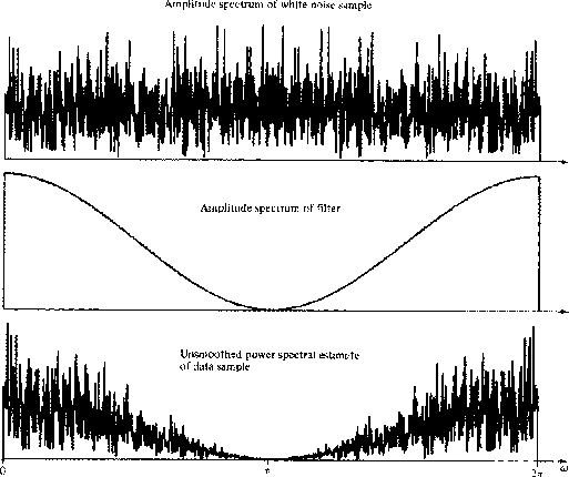
but, from the previous section, we learned that $E(\overline{X} X) = \sigma^2$.Considering $\sigma^2$ to be unity, we see that the expected power spectrum of the output Y is the energy spectrum of the filter F. The overall situation is depicted in Figure 6. The interesting question is how well can we estimate the spectrum when we start with an n-point sample of y_t. We will describe three computationally different methods, all having the same fundamental limitations.

 

4-5
Figure 6 Spectral estimation.

 

4-6
Figure 7 Spectral estimate of a random series.

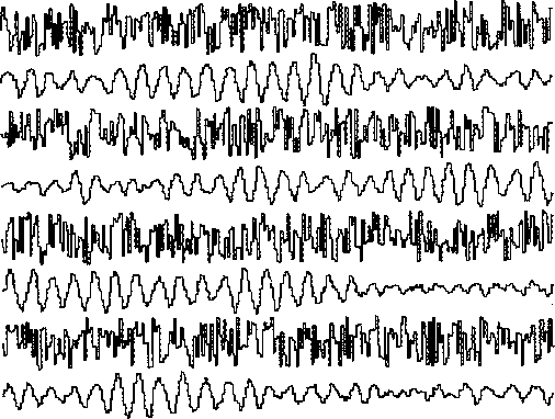
The first method uses a bank of filters as shown in Figure 7. When random numbers excite the narrowband filter, the output is somewhat like a sine wave. It differs in one important respect. A sine wave has constant amplitude, but the output of a narrowband filter has an amplitude which swings over a range. This is illustrated in Figure 8. If the bandwidth is narrow, the amplitude changes slowly. If the impulse response of the filter has duration $\Delta t_{\rm filter}$,then the output amplitude at time t will be randomly related to the amplitude at time $t + \Delta t_{\rm filter}$.Thus, in statistical averaging, it is not the number of time points but the number of intervals $\Delta t_{\rm filter}$which enhance the reliability of the average. Consequently, the decay time of the integrator $\Delta t_{\rm integrator}$will generally be chosen to be greater than $\Delta t_{\rm filter} = 1/\Delta f$.The variability $\Delta p$ of the output p decreases as $\Delta t_{\rm integrator}$ increases. Since v_t has independent values over time spans of about $\Delta t_{\rm filter} = 1/\Delta f$,then the ``degrees of freedom'' smoothed over can be written $\Delta t_{\rm integrator}/\Delta t_{\rm filter}=\Delta f\Delta t_{\rm integrator}$.The variability $\Delta p/p$ is proportional to the inverse square root of the number of degrees of freedom, and so we get

 

4-7
Figure 8 1024 random numbers before and after narrowband filtering. The filter was $(1- Z)/ ((1-Z/Z_{0})\, (1-Z/\overline{Z}_{0}))$where $Z_{0} = 1.02\, e^{i\pi/5}$.

$$\left( {\Delta p \over p} \right)^2 \eq {1 \over \Delta f \, \Delta t_{\rm integrator} }$$

or, introducing the usual inequality,  

$$\Delta t \, \Delta f\, \left( {\Delta p \over p}\right)^2 \quad\gt\quad 1$$ (52)

The inequality (52) indicates the three-parameter uncertainty which is fundamental to estimating power spectra of random functions. Two other methods of estimating the spectrum of y_t from a sample of length n are exactly the same as the methods described in Sec. 4-3 as ways of estimating the spectrum of white light. In fact, (52) turns out to be the same as (48).

The usual interpretation is that to attain a frequency resolution of $\Delta f$ and a relative accuracy of $\Delta p/p$ a time sample of duration at least $\Delta t \gt 1/[\Delta f\, (\Delta p/p)^2]$ will be required. Although this sort of interpretation is generally correct, it will break down for highly resonant series recorded for a short time. Then the data sample may be predictable an appreciable distance off its ends so that the effective $\Delta t$ is somewhat (perhaps appreciably) larger than the sample length.

EXERCISES:

1. It is popular to taper the ends of a data sample so that the data go smoothly to zero at the ends of the sample. Choose a weighting function and discuss in a semiquantitative fashion its effect on $\Delta t$, $\Delta f$,and $(\Delta p/p)^2$.
2. Answer the question of Exercise 1, where the autocorrelation function is tapered rather than the data sample.