Next: VTI homogeneous media
Up: Analytical Approximations of the
Previous: Analytical Approximations of the
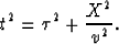
In order to evaluate the stationary point (the point in which the phase is minimum or maximum),
we need to solve the equation
|  |
(25) |
Equation (B-1) reduces to the condition that the horizontal projection for rays from each of
the source and receiver to the specular reflection point (SRP) add up to equal the source-receiver
offset, X (Popovici, 1995).
Solving equation (B-1) in its full form involves solving a
sixth-degree polynomial, which I prefer to avoid doing
analytically.
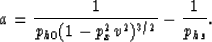
Setting px=0 in equation (B-1) yields solutions (stationary points) for reflections from
horizontal reflectors,
and, therefore, equation (B-1) reduces to
|  |
(26) |
with a stationary point given by
|  |
(27) |
In fact, ph0 is the exact stationary point solution for horizontal reflections,
which can be derived directly from the hyperbolic moveout equation:
Where 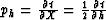 ,
,
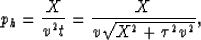
which is the same as equation (B-3).
Expanding equation (B-1) using Taylor's series around ph=0,
and ignoring terms beyond the linear in ph, yields
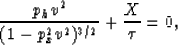
with a stationary point given by
|  |
(28) |
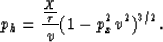
Equation (B-4) corresponds to the exact solution for a vertical reflector,
where ph=0 and  . It also provides a good approximation away
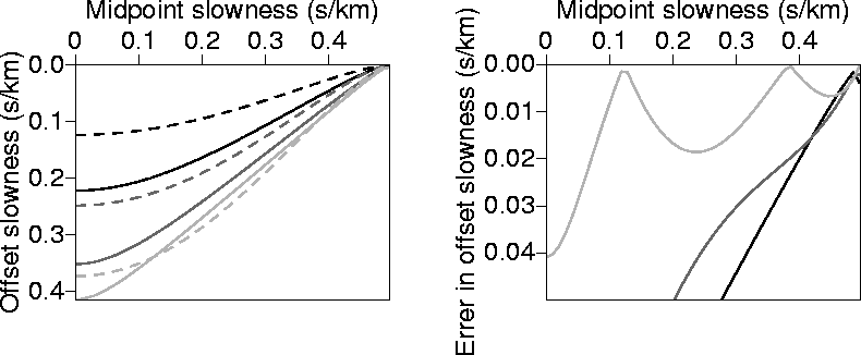
from . Figure B-1 shows a comparison between the exact ph solution of
equation (B-1) (obtained numerically)
and that given by equation (B-4) as a function of px for three sets of
. It also provides a good approximation away
from . Figure B-1 shows a comparison between the exact ph solution of
equation (B-1) (obtained numerically)
and that given by equation (B-4) as a function of px for three sets of  . The
absolute difference between the two solutions is also displayed. As expected, errors increase with
offset, and
ph1eta0m
. The
absolute difference between the two solutions is also displayed. As expected, errors increase with
offset, and
ph1eta0m
Figure 17 Left: Values of ph as a function px calculated numerically
(solid curves), and calculated analytically (dashed curves)using equation (B-4).
Right: The absolute difference
between the two curves on the left. The medium is homogeneous and isotropic with v=2.0 km/s.
The black curve corresponds to =1.0 km/s, the dark-gray curve corresponds to
=2.0 km/s, and the light gray curve corresponds to =3.0 km/s.

the accuracy
of the approximate solution reduces at px=0. In fact, for px=0, ph in
equation (B-4)
equals  which is clearly different from the exact solution given by
equation (B-3). Inserting the exact solution, in place of the factor
, in equation (B-4) yields a new approximate solution for ph given by
which is clearly different from the exact solution given by
equation (B-3). Inserting the exact solution, in place of the factor
, in equation (B-4) yields a new approximate solution for ph given by
| 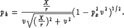 |
(29) |
This solution is exact for px=0 and , and therefore, I will refer
to it as the 2-point solution (it fits exactly at two points).
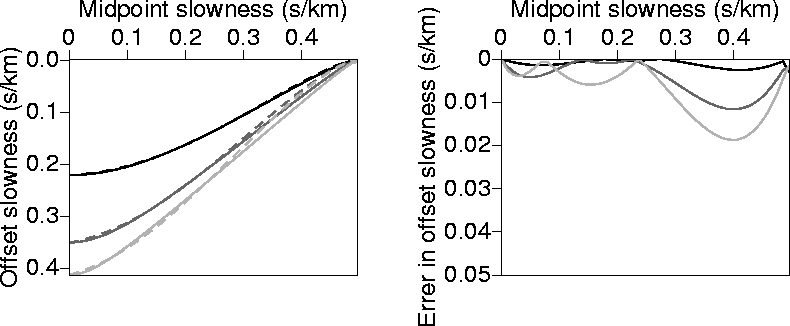
Figure B-2 shows a comparison
between the exact solution of equation (B-1) (obtained numerically)
and that given by equation (B-5), again for three sets of .Clearly, this new curve of ph better fits the exact solution than that given in Figure B-1.
Although
the percentage of error in ph seems to be high, the corresponding error in the phase estimate
(which is the key quantity used in the migration) is much lower
because  , as depicted in Figure 1,
is rather insensitive to ph, especially around the exact solution.
In other words, the curvature of the phase function around its minimum is low. Such low curvature, according
to equation (A-2), will result in a greater contribution in terms of amplitude.
This translates to practically
no error when it comes to actual geophysical applications.
ph2eta0m
, as depicted in Figure 1,
is rather insensitive to ph, especially around the exact solution.
In other words, the curvature of the phase function around its minimum is low. Such low curvature, according
to equation (A-2), will result in a greater contribution in terms of amplitude.
This translates to practically
no error when it comes to actual geophysical applications.
ph2eta0m
Figure 18 Same as in Figure B-1, but with the analytical solution evaluated
using the 2-point fitting of equation (B-5).
Let's find yet another exact solution,
that is, the solution when ps=0 (px=ph). The reflector angular
correspondence of this approximation depends on the offset. In this case,
equation (B-1) reduces to
| 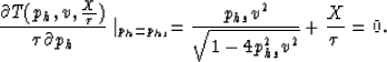 |
(30) |
with a solution for ph given by
|  |
(31) |
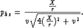
To insure that ph given by equation (B-5) has the value of phs
as px=ph, we must insert, some how, equation (B-7)
into equation (B-5). This task is accomplished by forcing ph,
given by equation (B-5), to linearly equal
phs at px=ph,
and, thus, equation (B-5) becomes
| ![\begin{displaymath}
p_h = \frac{\frac{X}{\tau}}{v \sqrt{(\frac{X}{\tau})^2 + v^2}} (1-p_x^2 v^2)^{3/2} [a(p_{hs})p_x+b].\end{displaymath}](img95.gif) |
(32) |
The term between the square brackets is to insure this linear fit.
To solve for a and b in equation (B-8), ph must satisfy two conditions:
(1) ph should reduce to the form given by equation (B-3) for px=0, and this condition
will result in b=1.
(2) ph should reduce to the form given by equation (B-7) for px=phs.
The second condition, after some mathematical manipulation, yields
Therefore, ph given by equation (B-8) is an exact solution of equation (B-1)
at three points (px=0, px=phs, and ) and a good approximation, as
demonstrated by Figure B-3, elsewhere. I will refer to this equation as the 3-point
solution.
Figure B-3 shows ph given by equation (B-8) next to the exact solution for ph.
Clearly, the three point fitting given by equation (B-8) resulted in a good approximation
of ph. The accuracy of this approximation will be better appreciated when we observe the low amount of
errors in traveltime calculation induced by this approximation (i.e., Figure 3).
ph3eta0m
Figure 19 Same as in Figure B-1, but with the analytical solution evaluated
using the 3-point fitting of equation (B-8).
Next: VTI homogeneous media
Up: Analytical Approximations of the
Previous: Analytical Approximations of the
Stanford Exploration Project
11/11/1997