Least-squares imaging and deconvolution using the hybrid norm conjugate-direction solver

Application - Deconvolution

Deconvolution has been a well-known geophysical problem since the 1950s. We investigate the spiking deconvolution, which aims to compress the source wavelet, such that a reflectivity series with higher resolution can be obtained. The simple convolution model is expressed as follows:

$$m(t)*s(t) + n(t) = d(t)$$ (3)

where r(t) is the reflectivity series, s(t) is the source wavelet, n(t) is random noise, and d(t) is the seismic traces (we assume a certain kind of amplitude compensation has already been applied).

Intrinsically, this is an under-determined problem, because both $r(t)$ and $s(t)$ are unknown. Further assumptions about the reflectivity series are needed in order to get a deterministic answer. In the L2 scenario, the underlying assumption is that the reflectivity model is purely random (i.e., has a white spectrum). As mentioned before, the model may in fact be spiky, which is better matched by an L1 type inversion. Therefore the hybrid result should outperform the L2 result.

For simplicity, we also assume that source wavelet is minimum phased. The conventional spiking deconvolution can be defined as an inverse problem,

$$\bold D \bold a \approx \bold 0 ,$$

where $\bf D$ is the data convolution operator, and $\bf {a}$ is the filter. In this formulation, the filter is the only unknown, and in theory the data residual itself is the reflectivity model.

To incorporate the model regularization into the inversion framework, we generalize the formulation above by posing the deconvolution problem as such inversion problem:

$$\left\{ \left[ \begin{array}{cc} \bold{D} & \bold{-I} \bold{0}... ...approx \left[ \begin{array}{c} \bold 0 \bold 0 \end{array} \right] \right. ,$$ (4)

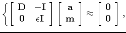in which $\bold D$ is the data convolution operator, $\bf {a}$ is the filter, and $\bf m$ is the reflectivity model. The parameter $\bf\epsilon$ indicates the strength of the regularization. Since the source wavelet is assumed to be a minimum-phase wavelet, ideally the inversion gives the exact inverse of the source wavelet to $\bold a$ .

The first equation in (4) (data fitting) implies that after convolving the data with the filter, we should get the reflectivity model; any values that cannot fit the reflectivity model are considered as noise in data. The second equation in (4) is the spiky regularization of the model; thus we apply the hybrid norm.

Least-squares imaging and deconvolution using the hybrid norm conjugate-direction solver