Least-squares imaging and deconvolution using the hybrid norm conjugate-direction solver

Numerical example

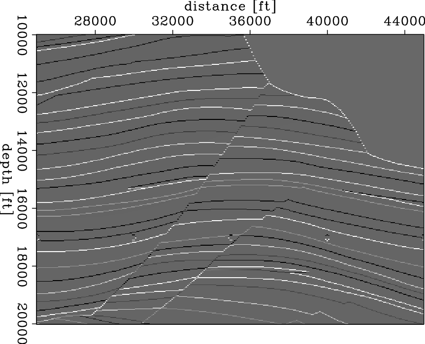
The reflectivity model we started with is a cropped subsalt region from the sigsbee2A reflectivity model, as shown in Figure 1(a). Notice that it is quite sparse.

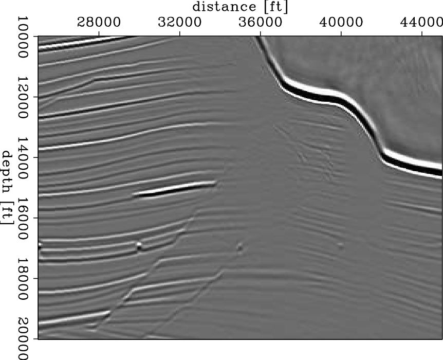
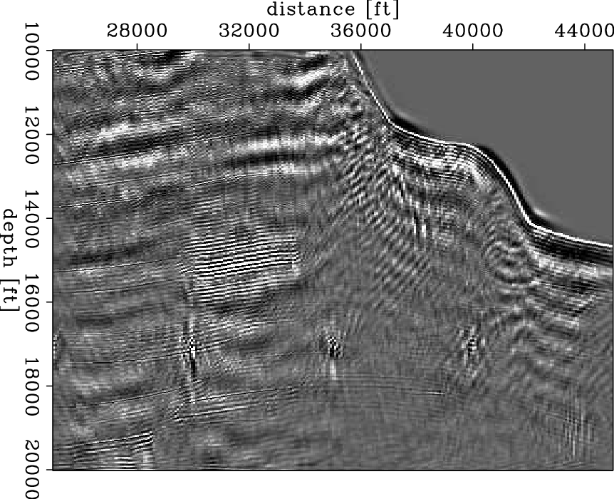
Figure 1(b) shows the input migrated image ${\bf m_{mig}}$ . While the data ${\bf d}$ is modeled with a two-way wave equation, both the migrated image ${\bf m_{mig}}={\bf L'd}$ and the Hessian operator are computed using a one-way wave-equation propagator. Therefore the data contains non-linear information (e.g., multiples) that cannot be resolved by the linearized one-way wave-equation operator. This explains some of the migration artifacts in the migrated image.

The explicit Hessian operator is computed using the receiver-side random-phase encoding method (Tang, 2008). The size of off-diagonal elements at each image point is $21 \times 21$ . After the Hessian is computed, we extract the portion corrsponds to the above reflectivity model.

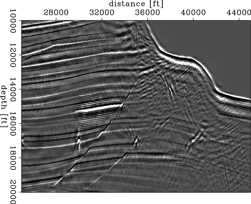
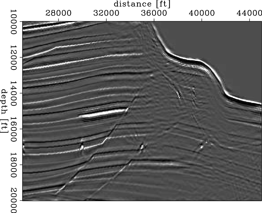
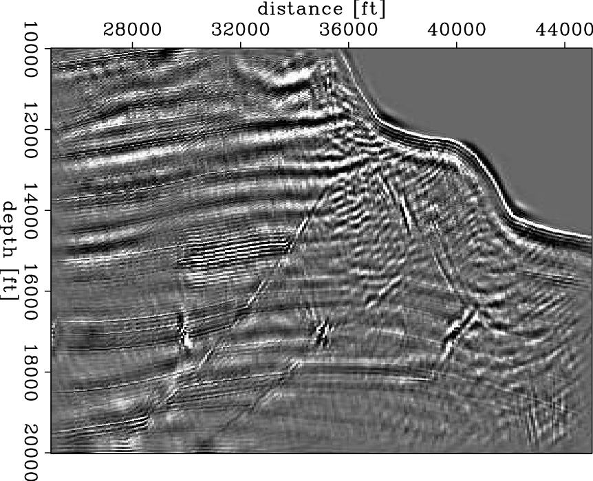
Figure 2(a) and 2(b) shows the inversion result of L2 and hybrid . The first thing to notice is that neither method can perfectly retrieve the original model; nonetheless, there is a significant improvement in the L1 inversion. The sharp boundary of the reflectors at the left of the image is better recovered in the hybrid result.

Figure 2(c) and 2(d) shows the data fitting errors of the two inversion are plotted. By evaluating the total energy of the fitting error (3.48% for both inversion results, $p_e={\bf \vert\vert Hm-m_{mig}\vert\vert _2/\vert\vert m_{mig}\vert\vert _2}$ ), we claim that hybrid inversion and L2 inversion fit the data almost equally well. This ensures that the major effect of the regularization is to fill the null space of ${\bf H}$ , with little effect on the data-fitting. However it is true that the data fitting residual of hybrid inversion appears to be more correlated to the reflectivity model than that of L2 inversion is.

refl-imaging,data-imaging-mig
Figure 1. (a) Reflectivity model; (b) input migrated image.

sigsb2a.mig.inv.l2,sigsb2a.mig.inv.hb,sigsb2a.mig.resd.l2,sigsb2a.mig.resd.hb
Figure 2. Comparison of the inversion results with L2 and hybrid regularization. (a): L2 inversion result; (b): hybrid inversion result; (c): L2 data fitting residual (d): hybrid data fitting residual.

In addition, notice that some parts of the sub-salt reflectors presented in the L2 result are missing in the hybrid result. The reason is clear: the hybrid norm is less tolerant of small values in the residual and always tries to put them down to zero (Claerbout, 2009b). This example shows that this feature of the hybrid norm is not always desirable.

Least-squares imaging and deconvolution using the hybrid norm conjugate-direction solver