|
 |
 |
 | Least-squares imaging and deconvolution using the hybrid norm conjugate-direction solver |  |
![[pdf]](icons/pdf.png) |
Next: Conclusion
Up: Application - Deconvolution
Previous: Deconvolution of a common-offset
It is not always true that wavelet can be extracted from the seismic
data, in this case we have to perform blind deconvolution.
To overcome the difficulty brought by non-minimum phase wavelet, we
turn back to the original non-linear convolution model
(3), and solve the non-linear inversion problem directly.
There are two ways to linearize this model. The first one is to use
model perturbation and neglect the non-linear higher order terms in the following:
in which
 are the initial model and source wavelet
respectively.
are the initial model and source wavelet
respectively.
 are the pertubation of them, the
linearized inversion will output
. The other way
of linearization is a two-stage linear least squares
formulation; i.e. alternately fixing one term (m or s) and inverting for
the other one. First use an initial
wavelet
are the pertubation of them, the
linearized inversion will output
. The other way
of linearization is a two-stage linear least squares
formulation; i.e. alternately fixing one term (m or s) and inverting for
the other one. First use an initial
wavelet  , keep
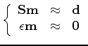
unchanged and invert for model m
, keep
unchanged and invert for model m
 |
(6) |
and then use the updated m to invert for wavelet s
 |
(7) |
Repeat this process (6) and (7) for several iterations.
As is in all non-linear inversion problems, the difficulty in these
methods is to find a good starting model. Another issue is to add
proper constrain on the wavelet
, for example, the wavelet should
have constant energy during inversion, but this constrain does not fit
the linear inversion framework.
|
|
|
|
| Least-squares imaging and deconvolution using the hybrid norm conjugate-direction solver | |
|
Next: Conclusion
Up: Application - Deconvolution
Previous: Deconvolution of a common-offset
2010-05-19