Interpolation

I now use another shot-gather, wz27 (Western Geophysical), also from Alaska. It also contains strong water-bottom multiples, but this is not the subject of this section. This shot-gather is interesting, because it contains 119 traces, but every other trace in the second half of the array is missing.

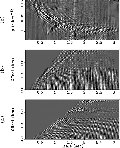
On Figure 4, I display the input shot-gather. I also represent the NMO-corrected data; the velocity analysis was again performed after a first attempt to remove of the water-bottom multiples in the $\tau-p$domain (Darche, 1990).

To perform the interpolation, I will first transform the data to the t₀-p domain. But, to compute the least-squares inverse of the modeling operator L, I will use an irregular space sampling, since I don't want to include the missing traces in the transform. I will apply equation (5) with the set of offsets of the real traces (94 traces at all). This is not the same as applying it to the regularly sampled gather, and considering the missing traces are filled with zeros: the inverse would try to reconstitute these zeros.

 

H27iinput
Figure 4 Shot-gather wz27. (a) Input data; dt=4 msec, 119 traces: in the last 60 last traces, every other trace is missing. (b) After NMO correction; the velocity analysis was performed after initial removal of the water-bottom multiples and peglegs. (c) Parabolic mapping; the missing traces are not taken into account in the transform, and the sampling is irregular. The far offsets are overweighted; using 94 traces in the time-offset domain, I take 60 p-parameters to have an overdetermined system.

In fact, I overweight the far offsets, to emphasize the interpolation process on the last traces. I will use a weighting matrix W identical at all frequencies, but in which the values w(h) are 1 in the first 60 traces, and 4 in the last traces, in the region where traces are missing. The corresponding values U(t₀,p) appear on Figure 4.

Notice on Figure 4 that it is difficult to separate the primaries and the multiples peaks in the t₀-p domain. Effectively, the lag of the multiples is more or less 100 msec, and the multiples are rather short-period multiples. This explains why we see both kinds of events around p=0. Once again, the water-bottom reflection does not focus at p=0, due to the stretching at far offsets. Actually, the problem is worse than on the wz24, because some linear events (direct arrivals and low-frequency oscillations) are present on the input: after NMO correction, they cannot be modeled as parabolas.

To perform the interpolation, I use the modeling operator with modified parameters: 119 traces, regularly sampled, so that the energy in the t₀-p domain is spread over the whole space domain. I apply an inverse NMO-correction to the processed data, and I display the results on Figure 5.

The interpolation result has several interesting features. First, as expected, the far offsets have been successfully interpolated, since the parabolic transform was overweighted in this region. This is true either for the hyperbolic events (primaries and multiples) or the linear events, as it can be seen on the residuals. However, the near traces have been slightly modified. Especially, they have been roughened, losing some lateral coherency. Once again, the choice of the weighting was reducing the role of these traces, and it is not surprising to see some variations.

Actually, the choice of the weights is quite subjective. Effectively, I said that the parabolic model is not reliable at far offsets, and overweighting the far offsets might seem contradictory. On the other hand, the curvature of a parabola is better determined at far offsets. So, there is a trade-off between these criteria. I noticed on this data set that, if I underweight the last traces, the events are not well restored, and they tend to disappear on the last traces. Moreover, some strong aliased features at far offsets appear with this kind of weighting.

Another point is that it could be preferable to suppress (by dip-filtering) from the beginning the linear events, which cannot be modeled as parabolas after NMO correction. If we keep them, they tend to spread their energy on a vast region of p-parameters.

In conclusion, the interpolation can be considered successful, in the sense that the missing traces have been efficiently restored. The choice of the weights matters, according to the purpose of the process: not disturbing the near traces (far offsets underweighted), or restoring precisely the far traces (far offsets overweighted). A trade-off is to choose an uniform weighting.

 

H27iresult
Figure 5 Interpolation result. (a) Input gather. (b) Interpolated gather; starting from the parabolic mapping of Figure 4, I come back to the time-offset domain, using a modeling operator with 119 offsets. (c) Difference between the input and the interpolated gathers.