Multiples elimination

I use here the wz24 (Western Geophysical) shot gather. It was recorded in Alaska, which explains a hard ocean floor, due to arctic conditions. This hard ocean floor creates strong water-bottom multiples.

 

H24input
Figure 1 Shot-gather wz24. (a) Input: dt=4 msec, 3 sec of data; 24 traces, distant of 65 meters. (b) After multiples elimination in the $\tau-p$ domain, with a Burg-type adaptive algorithm ($\lambda=0.98$). (c) after NMO correction of the input gather, using a velocity analysis performed on (b); mute applied on the last traces.

 

H24nmopar
Figure 2 Parabolic mapping of the NMO-corrected shot gather. I used 24 parameters p, so that the system is still overdetermined. I also superposed the boundary of the region limiting the multiples, in which I will put the values to 0.

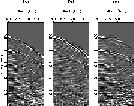
On Figure 1, I display the input shot gather, with the description of the recording parameters. The water-bottom multiples are easily visible: they are separated by lags of 0.5 seconds. Next to the input shot-gather, I also display a first attempt of removal of these multiples, with a method I describe in this report (Darche, 1990). It consists in doing a Burg-type adaptive processing in the $\tau-p$ domain, after a slant-stack transform. This process is especially useful to have a good estimate of the velocity curve of the primaries: a velocity analysis of the input gather only reveals velocity picks due to the strong multiples. However, I don't consider it as optimal in this case, because the multiples are not efficiently removed at far offsets. The velocity curve obtained from the first multiple removal enables us to perform the NMO correction of the input gather, and the result is also displayed on Figure 1.

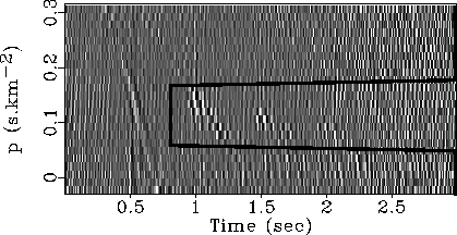
Then, I transform the NMO-corrected data to the t₀-p domain, applying the least-squares inverse (L^TL)^-1L^T in the frequency domain, with uniform weights. The advantage of this data-set is that the velocities of the primaries increase very rapidly with time, so that the multiples have far smaller velocities: their parabolic shape is more evident. The result is displayed on Figure 2, where I also mention the parameters of the transform.

On Figure 2, we can notice three basic topics. First, due to the stretch at far offsets, the water-bottom reflection does not focus around p=0, because of the stretch of the far-offsets after NMO correction. Then, the water-bottom multiples are clearly visible at 1 and 1.5 second, with two peaks around $p=0.1\ s.km^{-2}$. I isolated the region in which I find the multiples with a thick boundary line. Finally, no major event is visible after 2 seconds.

I isolate the water-bottom multiples by putting to 0 the values U(t₀,p) outside the corresponding region, described on Figure 2. The choice of the cut-off parameters is rather subjective, but is sufficient to prove the efficiency of the separation. I transform back the remaining values to the time-offset domain with the modeling operator L, and finally apply an inverse NMO correction. Thus, I obtain the field of multiples in the original shot-gather, as represented on Figure 3. The primary field is obtained by difference, and is also represented on Figure 3. You can also compare them with the results obtained by Zhang (1990; this report), who applied a migration scheme to remove the water-bottom multiples on the same shot-gather.

 

H24result
Figure 3 Separation of the multiples and primaries. (a) Input shot-gather (b) Field of the multiples. (c) Field of the primaries.

The multiples have been efficiently removed. Some major events, especially after 1.5 seconds, have been emphasized. I think a problem can come from the definition of the multiple region: if we take it too wide (in p), we localize the energy of the remaining events in a narrow band of the t₀-p domain, as though they were purely parabolic, and we could lose some amplitude-versus-offset information.

Finally, I advise not to work directly with the region defining the primaries on Figure 2. Effectively, it appears that the water-bottom reflection, especially, should be described by a wider range of p-parameters than the one I used: the modeling operator could not restitute it entirely, and it would be modified in the process. This is due in particular to the stretching at far-offsets, to the mute, and also to refracted arrivals. On the other hand, the multiples are known to be approximately parabolic, and their energy is concentrated in the region I defined, so we are sure to restitute them entirely.