Wave-equation migration velocity analysis by residual moveout fitting

Derivatives of moveout parameters ( ${\boldsymbol \mu}_{\vec x}$ ) with respect to slowness (${\bf {s}}$ )

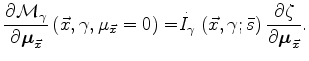
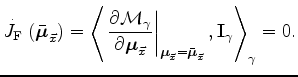
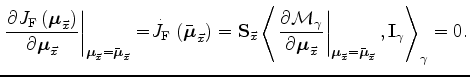
The evaluation of the derivatives of the moveout parameters with respect to slowness takes advantage of the fact that we need to evaluate the derivatives only at maxima for the objective function in equation 5. At the maxima, the objective function is stationary and thus its derivatives with respect to the moveout parameters are zero, and we can write:

$$\left. \frac {\partial {J_{\rm F}}\left({\boldsymbol \mu}_{\vec x... ...bar{{\boldsymbol \mu}}_{\vec x}}, {\bf I}_{\gamma } \right\rangle_{\gamma } =0.$$ (A-12)

As discussed above, the derivatives in the second term (II) of equation 9 are different from zero only when the moveout coefficient ${\mu_{\vec x}}$ and the image element share the same spatial coordinate. Consequently, for each ${\mu}_{\overline{x}}$ there is only one $\vec x$ for which the inner products above are different from zero. Equation 12 can thus be simplified into:

$$\stackrel{.}{{J_{\rm F}}}\left(\bar{{\boldsymbol \mu}}_{\vec x}\r... ...bar{{\boldsymbol \mu}}_{\vec x}}, {\bf I}_{\gamma } \right\rangle_{\gamma } =0.$$ (A-13)

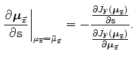
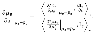
Using the rule for differentiating implicit functions, and taking advantage of the fact that the fitting problems are all independent from each other (i.e. the cross derivatives with respect to the moveout parameters are all zero), we can formally write:

$$\left. \frac {\partial {\boldsymbol \mu}_{\vec x}} {\partial {\bf... ...ft({\boldsymbol \mu}_{\vec x}\right) } {\partial {\boldsymbol \mu}_{\vec x}} }.$$ (A-14)

From equation 13 and 14, the derivative of the local moveout parameters with respect to slowness is:

$$\left. \frac {\partial {\boldsymbol \mu}_{\vec x}} {\partial {\bf... ...ar{{\boldsymbol \mu}}_{\vec x}}, {{\bf I}_{\gamma }} \right\rangle_{\gamma } }.$$ (A-15)

Appendix A presents the development for the expressions to compute the terms ${\partial^2 \mathcal M_{\gamma }}/{\partial {\boldsymbol \mu}_{\vec x}^2}$ (A-3), and ${\partial{\bf I}_{\gamma }}/{\partial {\bf {s}}}$ (A-5).

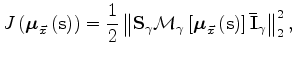
Combining the derivatives in equation 15 with the derivatives in equations 10-11 we can easily compute the gradient of the objective function 4 with respect to slowness that can be written, when $\bar{{\boldsymbol \mu}}_{\vec x}=0$ , as:

$$\nabla{{J}}= - \underbrace { \left( {\frac{\partial {{\bf P}_{s} ... ...\partial {\boldsymbol \mu}_{\vec x}^2} ' {{\bf\bar I_{\gamma }}} }. }_{\rm III}$$ (A-16)

I will now examine the effects of each of the terms in equation 16 starting from the rightmost one. The third term (III) produces a scalar for each local curvature parameter ${\mu_{\vec x}}$ . This scalar multiplies the image for each physical location after it has been differentiated in depth and scaled by ${\partial {\zeta}}/{\partial {\mu}_{\overline{x}}}$ , as described by the second term (II). Notice that the phase introduced by the depth derivative of the image in (II) is crucial for the successful backprojection into the slowness model that is accomplished by the first term (I). In this term, first ${\bf\Gamma}'$ transforms the image from the aperture-angle domain into the subsurface-offset domain. The transformed image is scaled, horizontally shifted, and spread across the shot axis by the application of ${\bar{{\bf P}}_{s} }'$ and ${\bar{{\bf P}}_{g} }'$ . Finally, the adjoint of operators $\frac{\partial {{\bf P}_{s} }}{\partial {\bf {s}}}'$ and $\frac{\partial {{\bf P}_{g} }}{\partial {\bf {s}}}'$ backproject the image perturbations into the slowness model along the source wavepaths and the receiver wavepaths, respectively.

Wave-equation migration velocity analysis by residual moveout fitting