|
|
|
|
Wave-equation migration velocity analysis by residual moveout fitting |
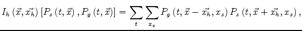
In wave-equation migration, as for example reverse-time migration,
the image is computed from the back-propagated receiver
wavefield,
![]() ,
and the forward-propagated source wavefield,
,
and the forward-propagated source wavefield,
![]() ,
where
,
where ![]() is the recording time,
is the recording time,
![]() is the model-coordinate vector,
is the model-coordinate vector,
![]() is the source position at the surface,
and
is the source position at the surface,
and
![]() is the slowness model.
is the slowness model.
The prestack image,
![]() ,
is computed as the zero lag of the
temporal cross-correlation between
the spatially-shifted
back-propagated receiver wavefield and
forward-propagated source wavefield
as
(Rickett and Sava, 2002):
,
is computed as the zero lag of the
temporal cross-correlation between
the spatially-shifted
back-propagated receiver wavefield and
forward-propagated source wavefield
as
(Rickett and Sava, 2002):
where
 is the half subsurface offset,
which in this paper I will assume to be horizontal,
but it does not need to be in the general case
(Biondi and Symes, 2004).
is the half subsurface offset,
which in this paper I will assume to be horizontal,
but it does not need to be in the general case
(Biondi and Symes, 2004).
The prestack image as a function of subsurface offset can be transformed to
an image as a function of reflection aperture angle,
![]() by using a linear operator
by using a linear operator
![]() (Sava and Fomel, 2003).
In matrix notation, if
(Sava and Fomel, 2003).
In matrix notation, if
![]() is a
is a
![]() matrix and
matrix and
![]() is a
is a
![]() matrix,
the image transformation from subsurface offset into the angle domain can be
expressed as:
matrix,
the image transformation from subsurface offset into the angle domain can be
expressed as:
I introduce an objective function
that maximizes the flatness of the angle-domain image
along the aperture-angle axis at all spatial locations ![]() .
This objective function aims at maximizing image flatness
not directly as a function of the slowness,
but indirectly through the application of an
angle-domain moveout operator
.
This objective function aims at maximizing image flatness
not directly as a function of the slowness,
but indirectly through the application of an
angle-domain moveout operator
![]() , which depends on the
column vector of
, which depends on the
column vector of
![]() moveout parameters
moveout parameters
![]() .
.
I define the application of the moveout operators
![]() to a prestack image computed by equations 1
and 2
with a background slowness
to a prestack image computed by equations 1
and 2
with a background slowness ![]() ,
as
,
as
| (A-3) |
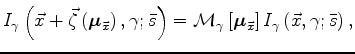 are the moveout shifts, assumed here to be simple depth shifts.
The operator
are the moveout shifts, assumed here to be simple depth shifts.
The operator
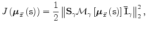
I further define the stacking operator
![]() that sums the image along the aperture-angle
axis
that sums the image along the aperture-angle
axis ![]() .
I can now introduce the objective function
that measures the flatness of the image as:
.
I can now introduce the objective function
that measures the flatness of the image as:
 is the slowness vector.
This objective function is not a direct function
of
,
but it depends on it indirectly through
the moveout parameters
is the slowness vector.
This objective function is not a direct function
of
,
but it depends on it indirectly through
the moveout parameters
The fitting problems maximize the zero lag
of the cross-correlation between the prestack image computed
for a realization of the slowness vector
and
the moved-out image computed with the background slowness
![]() .
For the sake of keeping the notation as compact as possible,
I combine the
.
For the sake of keeping the notation as compact as possible,
I combine the
![]() independent
fitting problems into one by defining the following objective function:
independent
fitting problems into one by defining the following objective function:
The vector of moveout parameters is therefore the solutions of the following maximization problem:
For velocity estimation in the angle domain,
an effective parametrization of the moveout
is the "curvature"
![]() ,
that defines the following moveout equation
,
that defines the following moveout equation
is equal to the background slowness
)
|
|
|
|
Wave-equation migration velocity analysis by residual moveout fitting |