Target-oriented least-squares migration/inversion with sparseness constraints

regularization with sparseness constraints

Inverting the linear system defined by equation 4 is difficult, because it is underdetermined due to the incomplete subsurface illumination caused by the limited surface acquisition and complex overburden. Another difficulty arises when our Born modeling operator ${\bf L}$ is not sufficient to model all the complexities in the observed data ${\bf d}_{\rm obs}$. For example, the commonly used one-way wave-equation propagator is based on acoustic assumption and cannot handle waves beyond $90$ degrees; its amplitude is also not accurate for wide angles propagations (Zhang et al., 2005). The operator mismatch can make the inversion unstable. Of course, adding more data and using more accurate modeling operators can always help, but a more cost effective way would be introducing regularization operators that impose the a priori information to stabilize the inversion and make it converge to a geologically reasonable solution. A widely used regularization is the $\ell _2$-norm damping, which minimizes the energy of the model parameters by introducing a secondary objective function, and the overal objective function to minimize becomes

$$J({\bf m}) = \vert\vert{\bf H m} - {\bf m}_{\rm mig}\vert\vert _2^2 + \epsilon \vert\vert{\bf m}\vert\vert _2^2,$$ (7)

where $\epsilon$ is a trade-off parameter that controls the strength of regularization. The $\ell _2$-norm damping assumes the statistic of the reflectivity has a Gaussian distribution, which often leads to a relatively smooth solution. If we assume that the reflectivity is made up of spikes (Oldenburg et al., 1981), then the short-tailed Gaussian distribution assumption becomes unappropriate. To obtain a spiky or sparse solution, a long-tailed distribution such as exponential (the $\ell_1$ norm) or Cauchy (the Cauchy norm) distribution should be used (Sacchi and Ulrych, 1995). The objective function with a regularization in the Cauchy norm reads

$$J({\bf m}) = \vert\vert{\bf H m} - {\bf m}_{\rm mig}\vert\vert _2^2 + \epsilon S({\bf m}),$$ (8)

where $S({\bf m})$ is a non-quadratic regularization function defined as follows:

$$S({\bf m}) = \sum_{\bf x}{\rm log}(1+m^2({\bf x})/\sigma^2),$$ (9)

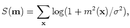
in which $\sigma^2$ is a scalar parameter of the Cauchy distribution that controls the sparsity of the model. The objective function 8 can be minimized under $\ell _2$ norm with the iterative reweighted least-squares (IRLS) technique (Nichols, 1994; Darche, 1989; Guitton, 2000; Scales and Smith, 1994), which equivalently minimizes the following non-linear objective function:

$$J({\bf m}) = \vert\vert{\bf H m} - {\bf m}_{\rm mig}\vert\vert _2^2 + \epsilon\vert\vert{\bf Q}{\bf m}\vert\vert _2^2,$$ (10)

where ${\bf Q}$ is a model dependent diagonal operator defined as follows:

$${\bf Q} = {\rm\bf diag}\left(\frac{1}{\sqrt{1+m^2({\bf x})/\sigma^2}}\right).$$ (11)

The detailed implementation of IRLS can be found in Nichols (1994); Darche (1989); Guitton (2000); Scales and Smith (1994).

Target-oriented least-squares migration/inversion with sparseness constraints