Target-oriented least-squares migration/inversion with sparseness constraints

Target-oriented least-squares migration

Within limits of the Born approximation of the acoustic wave equation, the seismic data can be modeled with a linear operator as follows

$${\bf d} = {\bf L m},$$ (1)

where ${\bf d}$ is the modeled data, ${\bf L}$ is the Born modeling operator and ${\bf m}$ denotes the reflectivity of the subsurface (a perturbed quantity from the background velocity). The simplest way is to use the adjoint of the Born modeling operator to image the reflectivity ${\bf m}$ as follows:

$${\bf m}_{\rm mig} = {\bf L}'{\bf d}_{\rm obs},$$ (2)

where the superscript denotes the conjugate transpose and the subscript $_{\rm obs}$ denotes observed data. However, migration produces unreliable images in areas of poor illumination. To get an optimally reconstructed image, we can invert equation 1 in the least-squares sense. The least-squares soltuion of equation 1 can be formally written as follows

$${\bf m} = {\bf H}^{-1}{\bf m}_{\rm mig},$$ (3)

where ${\bf H}={\bf L}'{\bf L}$ is the Hessian operator. Equation 3 has only symbolic meaning, because the Hessian is often singular and its inverse is not easy to obtain directly. A more practical method is to reconstruct the reflectivity ${\bf m}$ through iterative inverse filtering by minimizing a model-space objective function defined as follows:

$$J({\bf m}) = \vert\vert{\bf Hm}-{\bf m}_{\rm mig}\vert\vert _2^2,$$ (4)

where $\vert\vert\cdot\vert\vert _2$ denotes the $\ell _2$ norm. Each component of the Hessian matrix ${\bf H}$ can be computed with the following equation, which is obtained by evaluating the operator ${\bf L}'{\bf L}$ (Plessix and Mulder, 2004; Valenciano, 2008):

$$H({\bf x},{\bf y}) = \sum_{\omega}\omega^4\sum_{{\bf x}_s}\vert f_s(\omega)\vert^2G({\bf x},{\bf x}_s,\omega)G'({\bf y},{\bf x}_s,\omega)$$

$$\times \sum_{{\bf x}_r}w({\bf x}_r,{\bf x}_s)G({\bf x},{\bf x}_r,\omega)G'({\bf y},{\bf x}_r,\omega),$$ (5)

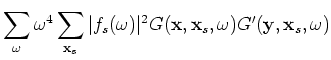
where ${\omega}$ is the angular frequency, and $f_s(\omega)$ is the source function; $G({\bf x},{\bf x}_s,\omega)$ and $G({\bf x},{\bf x}_r,\omega)$ denote Green's functions connecting the source location ${\bf x}_s=(x_s,y_s,0)$ and receiver location ${\bf x}_r=(x_r,y_r,0)$ to the image point ${\bf x}$, respectively. We have similar definitions for $G({\bf y},{\bf x}_s,\omega)$ and $G({\bf y},{\bf x}_r,\omega)$, except that they define the Green's functions connecting the source and receiver locations to another image point ${\bf y}$ in the subsurface. Throughout this paper, we assume the Green's functions are computed by means of one-way wavefield extrapolation (Stoffa et al., 1990; Claerbout, 1985; Ristow and Rühl, 1994). But Green's functions obatined with other methods, such as the ray-based approach, the two-way wave-equation-based approah and etc., can also be used under this framework. The weighting factor $w({\bf x}_s,{\bf x}_r)$ denotes the acquisition mask matrix (Tang, 2008a) defined as follows:

$$w({\bf x}_r,{\bf x}_s) = \left\{ \begin{array}{ll} 1 & \mbox{ if ... ...range of a shot at } {\bf x}_s; \\ 0 & \mbox{ otherwise }. \end{array} \right.$$ (6)

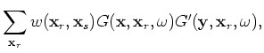
When ${\bf x}={\bf y}$, we obtain the diagonal elements of the Hessian; when ${\bf x}\neq{\bf y}$, we obtain the off-diagonal elements. A target-oriented truncated Hessian is obtained by computing the Hessian for ${\bf x}$'s that are within the target zone and a small number of ${\bf y}$'s that are close to each ${\bf x}$ (Valenciano, 2008).

Target-oriented least-squares migration/inversion with sparseness constraints