Target-oriented least-squares migration/inversion with sparseness constraints

numerical examples

I test both regularized target-oriented inversion schemes (equation 7 and 8) on the Marmousi model. Two data sets are synthesized: the first one is generated using one-way wave-equation Born modeling, while the second one is generated using two-way acoustic wave-equation finite-difference modeling. Figure 3(a) shows the stratigraphic velocity model used for the two-way wave-equation modeling. Figure 3(b) and Figure 3(c) show the corresponding background velocity model (the low frequency component of Figure 3(a)) and the reflectivity model (the high frequency component of Figure 3(a)) for the one-way wave-equation Born modeling. For both data sets, I model $251$ shots ranging from $4000$ m to $9000$ m with a $20$ m sampling. The receiver spread is fixed for all shots and spans from $4000$ m to $9000$ m with a $10$ m sampling. Figure 4 compares the modeled shot gathers located at $6500$ m. Note the amplitude differences between both data. Also note that some complexities present in two-way finite-difference modeled data are not modeled using the one-way Born modeling.

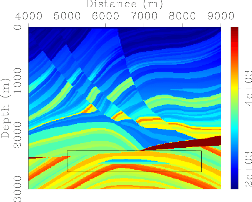
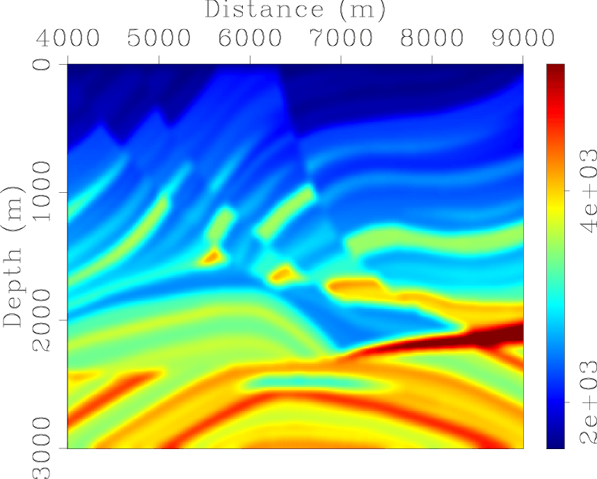
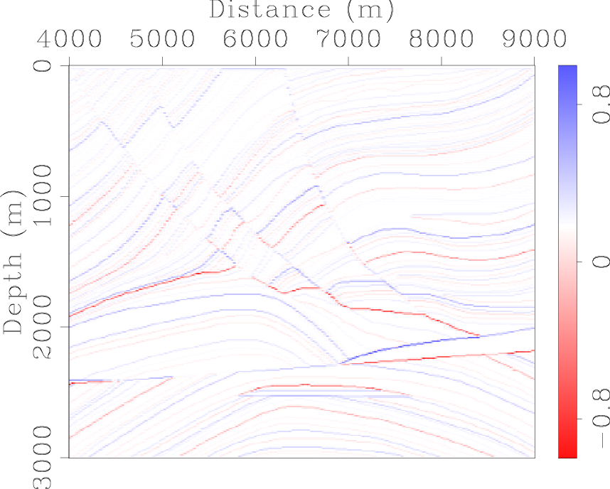
marm-vmod-stra,marm-vmod,marm-refl
Figure 3. The Marmousi model. Panel (a) is the stratigraphic velocity model used for two-way wave-equation finite-difference modeling. Panels (b) and (c) are the background velocity model and reflectivity model used for one-way wave-equation Born modeling. [ER]

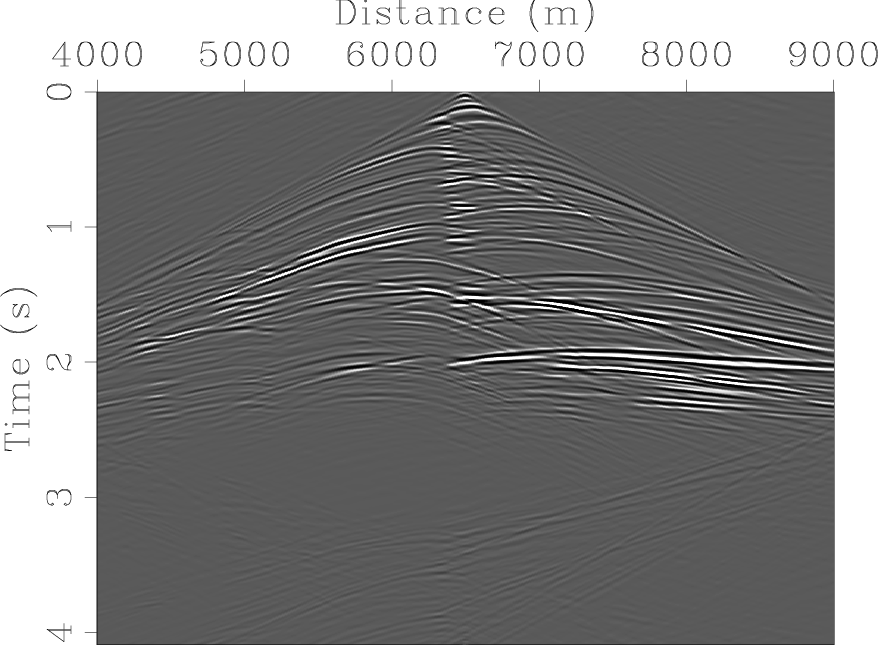
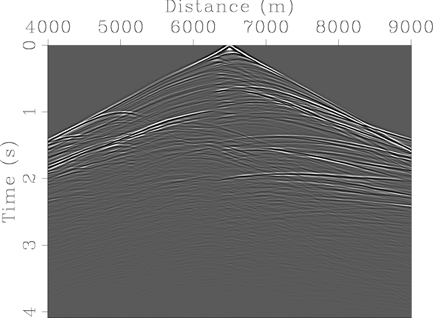
marm-trec-one-way,marm-trec-two-way
Figure 4. Comparison between shots synthesized using (a) one-way wave-equation Born modeling and (b) two-way wave-equation finite-difference modeling. [CR]

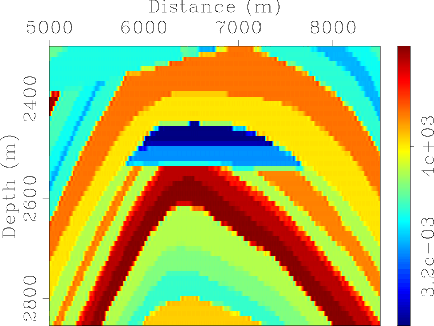
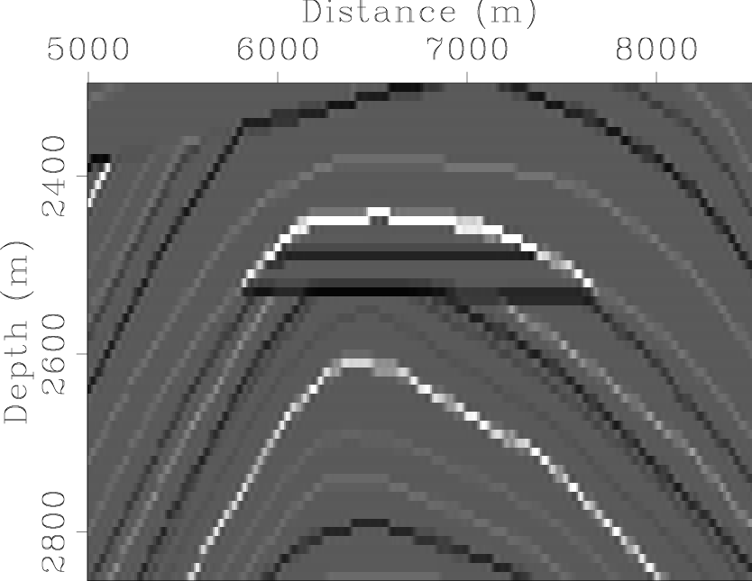
The target zone selected for inversion tests is outlined with a small box in Figure 3(a), a close-up look is also shown in Figure 5(a). The target zone is where the reservoir locates. The target-oriented Hessian is computed using the receiver-side random-phase encoding (Tang, 2008a,b). The smooth background velocity model (Figure 3(b)) and the Fourier finite-difference (FFD) one-way extrapolator (Ristow and Rühl, 1994) are used for migrating both one-way and two-way data and also for the Hessian computation. 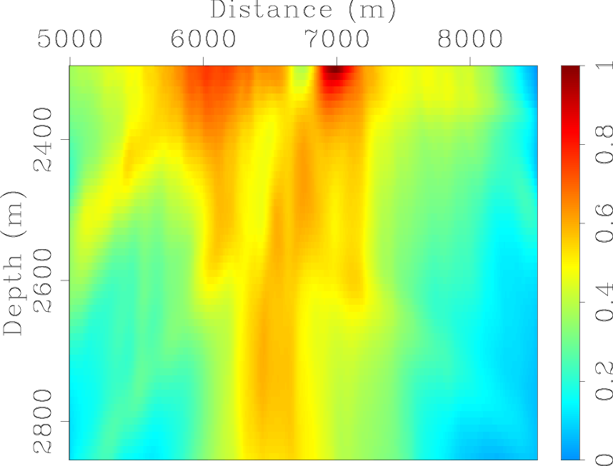Figure 5(b) illustrates the diagonal elements of the phase-encoded Hessian for the target area (the amplitude is normalized). Note the uneven illumination due to the limited acquisition geometry and complex velocity model. 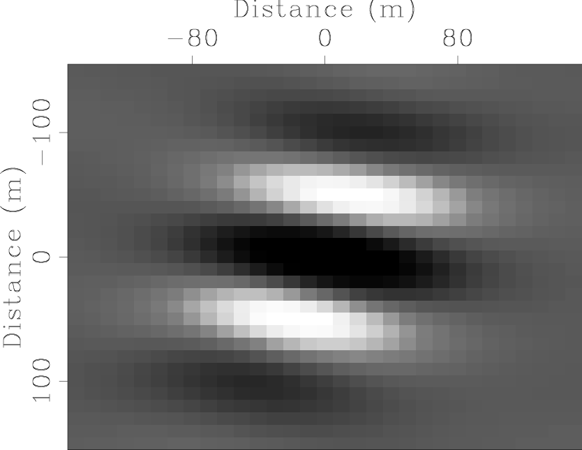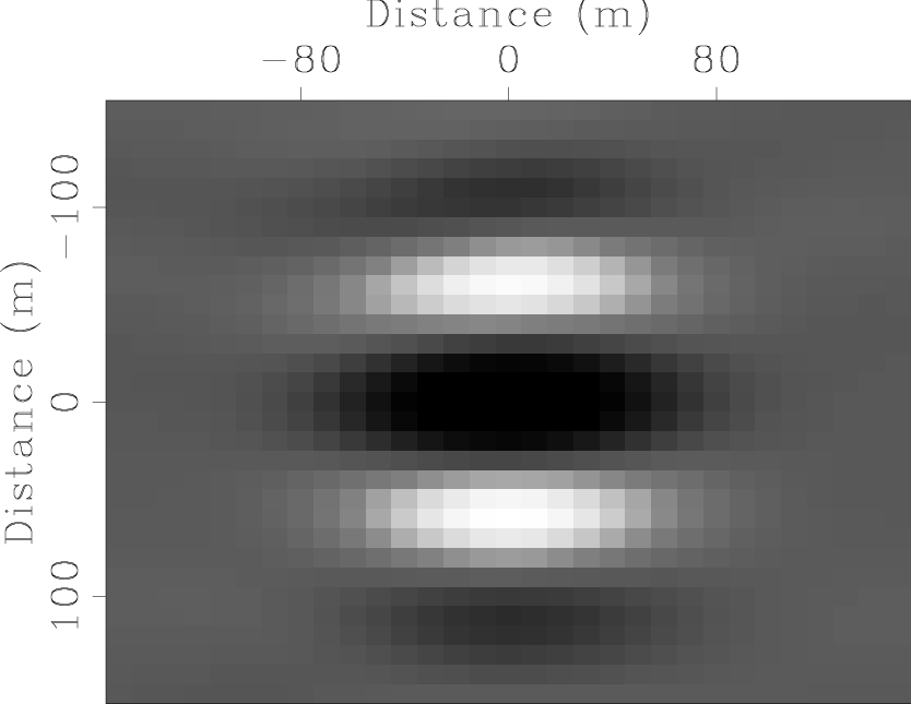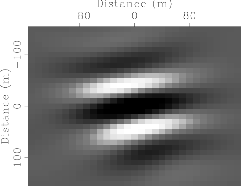Figure 6 shows the truncated local Hessian filters for three different image points (three rows of the truncted Hessian). The size of the filter is $31\times31$ in $x$ and $z$ directions, which seems to be big enough to capture most of the energy in the Hessian matrix.

marm-stra-target,marm-hess-diag-target
Figure 5. (a) The stratigraphic velocity model for the target zone. (b) The diagonal of the Hessian for the target zone. [CR]

marm-hess-offd-target-1,marm-hess-offd-target-2,marm-hess-offd-target-3
Figure 6. The local Hessian filters at (a) $x=5250$ m, $z=2800$ m, (b) $x=6500$ m, $z=2600$ m and (c) $x=8400$ m, $z=2400$ m. [CR]

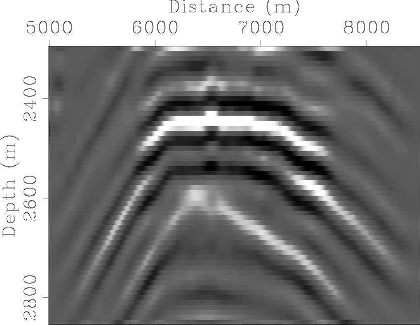
Figure 7 shows the inversion results on the one-way wave-equation Born-modeled data. This example represents the ideal case for one-way wave-equation inversion, since our modeling operator can "explain" all the physics present in the "observed" data (Figure 4(a)). As expected, migration produces a blurred image (Figure 7(b)); the regularized inversion schemes optimally deblur the migrated image, and the reflectivity is better recovered (Figure 7(c) and Figure 7(d)). Note that both inversion schemes enhance the spatial resolution. Also note that regularization with the sparseness constraint produces slightly higher resolution than regularization with the standard $\ell _2$-norm damping and Figure 7(d) is closer to the true reflectivity shown in Figure 8(a). This suggests that the sparseness constraint better predicts the model covariance, so that it more effectively reduces the null space and provides more accurate inversion result.

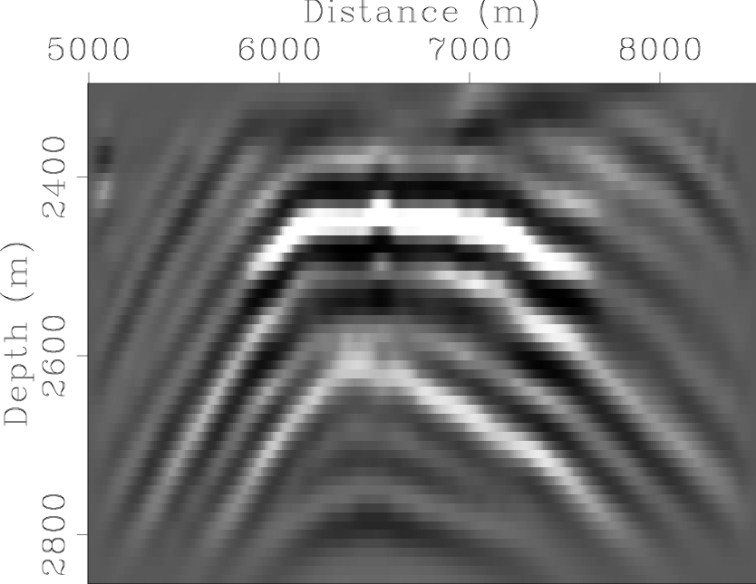
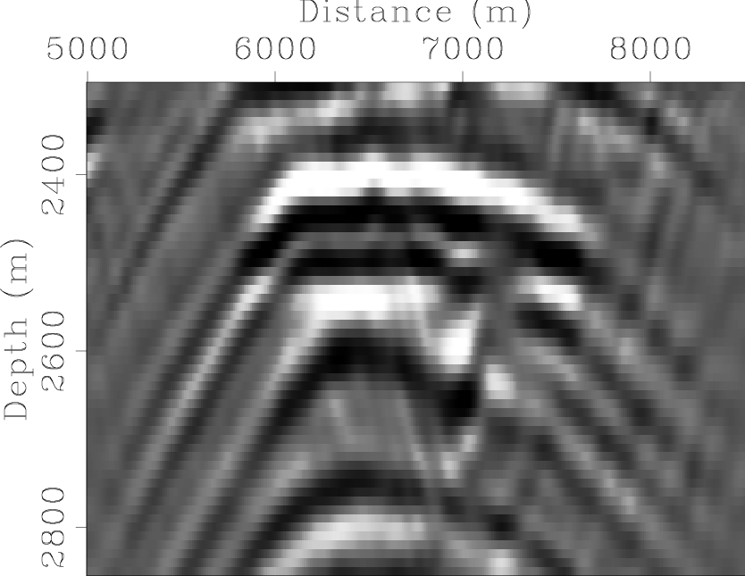
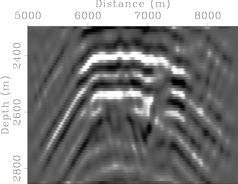
More interesting and also more instructive examples are shown in Figure 8, where both regularized inversion schemes are applied to the data synthesized using the two-way wave-equation finite-difference modeling (Figure 4(b)). In this case, the one-way wave-equation migrated image (Figure 8(b)) is much noisier than the corresponding result using the one-way Born data (Figure 7(b)); the amplitudes are also more distorted. This phenomenon is due to the operator mismatch, where the internal multiples and wide angle propagations cannot be modeled by the one-way Born modeling operator. Consequently, they contribute to the artifacts shown in Figure 8(b). 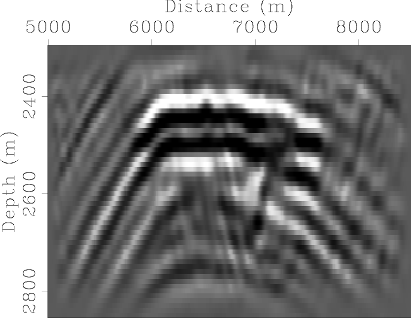The operator mismatch also influences the inversion results, as shown in Figure 8(c) and Figure 8(d). The inverted images are noisier and have more artifacts compared to the results obtained on the one-way Born data. But noticeable improvement on resolution over migrated image (Figure 8(b)) can still be identified. Note that inversion regularized with the sparseness constraint seems to provide a less noisy image with slightly higher spatial resolution than the inverted image regularized with the $\ell _2$-norm damping. This example suggests that when we have operator mismatch issues for inverse problems, it is important to add regularization operators that more accurately predict the model covariance. In this particular example, although promoting sparsity may not be the best regularization, it does better predicts the model covariance than the $\ell _2$-norm damping, hence it produces a better result even when our operator is not able to fully explain the observed data.

marm-refl-target,marm-imag-one-way-target,marm-invt-one-way-target-l2,marm-invt-one-way-target-l1
Figure 7. Target-orineted inversion of the one-way wave-equation Born-modeled data. (a) The true reflectivity, (b) migration, (c) inversion regularized with $\ell _2$ norm damping (equation 7) and (d) inversion regularized with the sparseness constraint (equation 8). [CR]

marm-refl-target,marm-imag-two-way-target,marm-invt-two-way-target-l2,marm-invt-two-way-target-l1
Figure 8. Target-orineted inversion of the two-way wave-equation finite-difference modeled data. (a) The true reflectivity, (b) migration, (c) inversion regularized with $\ell _2$ norm damping (equation 7) and (d) inversion regularized with the sparseness constraint (equation 8). [CR]

Target-oriented least-squares migration/inversion with sparseness constraints