migration imaging and inversion imaging as a least-squares problem

Seismic-wave imaging can be expressed as a least-squares inversion problem,  

$$min\vert\textbf{d}^{cal}-\textbf{d}^{obs}\vert ^{2},$$ (33)

where, given an underground geological model characterized with some parameters such as P-wave velocity, S-wave velocity, and/or density, or a reflectivity image, we then create a synthetic data set which minimizes the "distance" between the calculated data set and the observed data set.

The solution of the inverse problem is expressed as follows:

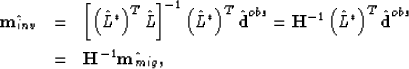$$\begin{eqnarray} \hat{\textbf{m}_{inv}}&=&\left[\left( \hat{L}^{*}\right)^{T}\ha... ...{d}}^{obs} \\ \nonumber &=&\textbf{H}^{-1}\hat{\textbf{m}_{mig}},\end{eqnarray}$$ (34)

or

$$\begin{eqnarray} \hat{\textbf{m}_{inv}}&=&\left[\left( \hat{L}^{*}\right)^{T}\ha... ...{d}}^{reg} \\ \nonumber &=&\textbf{H}^{-1}\hat{\textbf{m}_{mig}},\end{eqnarray}$$ (35)

or

$$\begin{eqnarray} \hat{\textbf{m}_{inv}}&=&\left[\left( \hat{L}^{*}\right)^{T}\ha... ...}}^{datum} \\ \nonumber &=&\textbf{H}^{-1}\hat{\textbf{m}_{mig}}.\end{eqnarray}$$ (36)

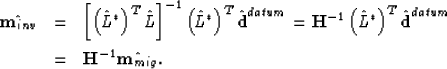
Similarly, if we assume Hessian matrix is a unitary matrix, equation (), (), and () all degenerate to  

$$\hat{\textbf{m}_{mig}}=\left( \hat{L}^{*}\right) ^{T}\hat{\textbf{d}}^{obs}.$$ (37)

Migration imaging avoids the matrix inversion by replacing the general inverse with a conjugate-transpose operator $\left( \hat{L}^{*}\right) ^{T}$. The advantage of the processing is to change an ill-posed inverse problem into a well-posed wavefield backpropagation problem, which is quite stable and robust (, , , ). In fact, migration imaging mainly locates the reflector and gives only a qualitative estimate of the reflectivity. $\left( \hat{L}^{*}\right) ^{T}$ is the two-way or one-way propagator, which commonly is expressed in the form of the conjugate Green's function.

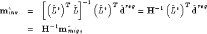
In fact, the quantitative estimation of the reflectivity should take advantage of inverse imaging. If we consider the reflectivity imaging as a weighting summation, equation () gives an unsuitable weight function. () discuss in detail about how to choose a suitable weight function.

The inverse of the Hessian matrix is just a deconvolution operator, which modifies the unsuitable weight function of the migration imaging. Therefore, equation () can give more accurate estimate of the reflectivity than can the migration imaging (equation ().

If equation () is rewritten as  

$$\hat{\textbf{m}}_{inv}=\textbf{H}^{-1} \hat{\textbf{m}}_{mig},$$ (38)

it is clear that Hessian matrix is a deconvolution operator, which improves the resolution of migration results (). We will consider how to quantitatively estimate the reflectivity with inverse imaging and determine the conditions under which direct inverse imaging and iterative inverse imaging are equivalent.