

Next: 3-D Theory \label>chapter:theory3d>
Up: 2-D Field Data Results
Previous: Playing Devil's Advocate: What
In this section I test the nonlinear iteration outlined in section
![[*]](http://sepwww.stanford.edu/latex2html/cross_ref_motif.gif) on the Mississippi Canyon data. I ran only one
nonlinear iteration. Since the velocity model is already quite nicely
determined, I did not do residual velocity analysis after the first run of
LSJIMP. However, I did recompute the crosstalk weights and the reflection
coefficients for each of the four multiple generators.
on the Mississippi Canyon data. I ran only one
nonlinear iteration. Since the velocity model is already quite nicely
determined, I did not do residual velocity analysis after the first run of
LSJIMP. However, I did recompute the crosstalk weights and the reflection
coefficients for each of the four multiple generators.
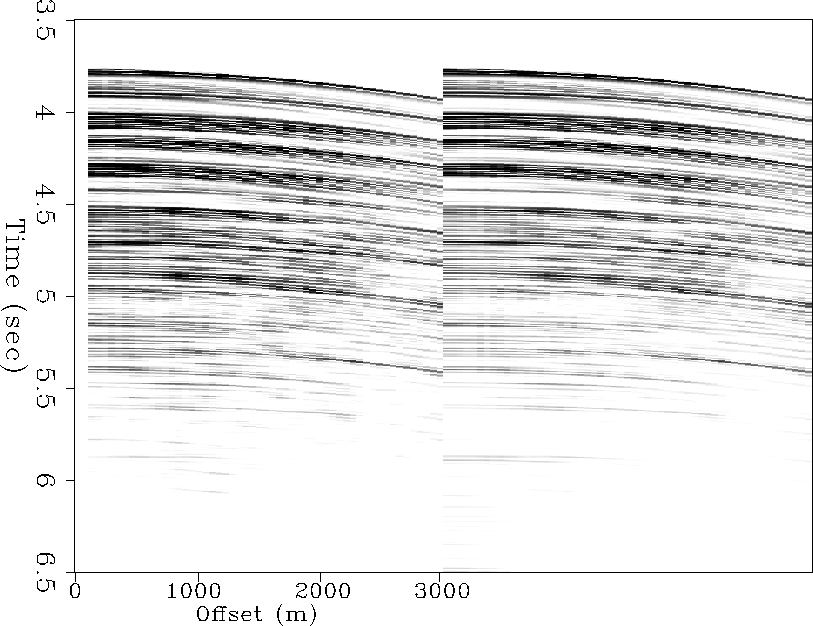
The updated crosstalk weights are shown in Figure ![[*]](http://sepwww.stanford.edu/latex2html/cross_ref_motif.gif) ,
at CMP 55 of 750. The most notable difference after the nonlinear update is the
infill of the near offsets. Although invisible in this case, the nonlinear
update also allows us to model crosstalk energy below twice the onset of the
first seabed multiple, which would be 7.5 seconds. This ability is very
important for data recorded in shallower water.
,
at CMP 55 of 750. The most notable difference after the nonlinear update is the
infill of the near offsets. Although invisible in this case, the nonlinear
update also allows us to model crosstalk energy below twice the onset of the
first seabed multiple, which would be 7.5 seconds. This ability is very
important for data recorded in shallower water.
crosstalk.gulf.iter
Figure 29
Crosstalk weights at CMP 55 of 750, before and after one nonlinear update.
Left: Crosstalk weights before update. Right: Crosstalk weights after update.
![[*]](http://sepwww.stanford.edu/latex2html/movie.gif)


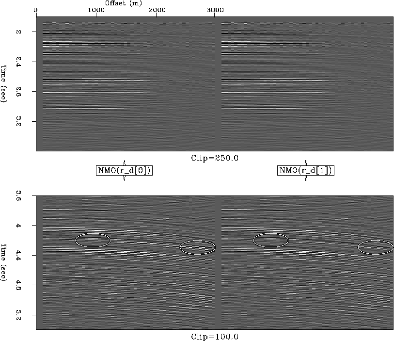
Figure ![[*]](http://sepwww.stanford.edu/latex2html/cross_ref_motif.gif) compares the weighted data residual at CMP 55
of 750 before and after the nonlinear update. The Figure is split in half along
the time axis as explained earlier in section
compares the weighted data residual at CMP 55
of 750 before and after the nonlinear update. The Figure is split in half along
the time axis as explained earlier in section ![[*]](http://sepwww.stanford.edu/latex2html/cross_ref_motif.gif) . The
most striking differences are highlighted with ovals. As mentioned earlier, the
R1 pure multiple and R2 seabed pegleg overlap over most of the 2-D line, which
inhibits estimation of R1's reflection coefficient. Although I do not show the
updated R1 reflection coefficient, Figure
. The
most striking differences are highlighted with ovals. As mentioned earlier, the
R1 pure multiple and R2 seabed pegleg overlap over most of the 2-D line, which
inhibits estimation of R1's reflection coefficient. Although I do not show the
updated R1 reflection coefficient, Figure ![[*]](http://sepwww.stanford.edu/latex2html/cross_ref_motif.gif) implicitly
illustrates the beneficial change. The event highlighted in ovals on the
residual panels, which has three visible peaks, does not have that wavelet shape
in the raw data. Crosstalk between the overlapping events and an improperly
high R1 reflection coefficient cause the event to be ``manufactured'' in the
LSJIMP result. By better estimating the R1 reflection coefficient, the event is
not present in the residual, and thus, not manufactured by LSJIMP. Other that
this event, however, the differences between the two panels are minimal.
implicitly
illustrates the beneficial change. The event highlighted in ovals on the
residual panels, which has three visible peaks, does not have that wavelet shape
in the raw data. Crosstalk between the overlapping events and an improperly
high R1 reflection coefficient cause the event to be ``manufactured'' in the
LSJIMP result. By better estimating the R1 reflection coefficient, the event is
not present in the residual, and thus, not manufactured by LSJIMP. Other that
this event, however, the differences between the two panels are minimal.
resd-iter1.gulf
Figure 30
LSJIMP data residual before and after nonlinear update of crosstalk weights
and reflection coefficients. Left: residual before updating. Right: residual
after updating. Panels split in half along time axis for display purposes and
clipped as labeled.
![[*]](http://sepwww.stanford.edu/latex2html/movie.gif)


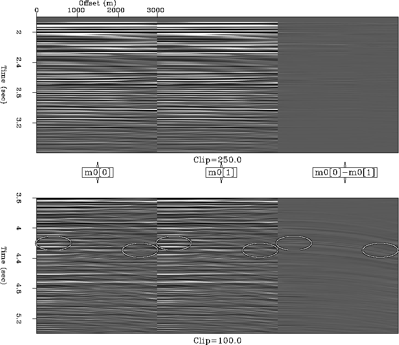
Figure ![[*]](http://sepwww.stanford.edu/latex2html/cross_ref_motif.gif) compares the LSJIMP estimated primaries at CMP
55 of 750 before and after the nonlinear update. The Figure is split in half
along the time axis as explained earlier in section
compares the LSJIMP estimated primaries at CMP
55 of 750 before and after the nonlinear update. The Figure is split in half
along the time axis as explained earlier in section ![[*]](http://sepwww.stanford.edu/latex2html/cross_ref_motif.gif) .
Ovals highlight the same regions as were highlighted in Figure
.
Ovals highlight the same regions as were highlighted in Figure
![[*]](http://sepwww.stanford.edu/latex2html/cross_ref_motif.gif) . The differences between the two estimated primary
panels are quite subtle; the difference panel on the right is more
englightening. Notice how the manufactured event discussed earlier is better
suppressed after the nonlinear update.
. The differences between the two estimated primary
panels are quite subtle; the difference panel on the right is more
englightening. Notice how the manufactured event discussed earlier is better
suppressed after the nonlinear update.
model-iter1.gulf
Figure 31
LSJIMP estimated primaries before and after nonlinear update of crosstalk
weights and reflection coefficients. Left:  before updating.
Center:
  after updating. Right: Difference. Panels split in half
along time axis for display purposes and clipped as labeled.
![[*]](http://sepwww.stanford.edu/latex2html/movie.gif)


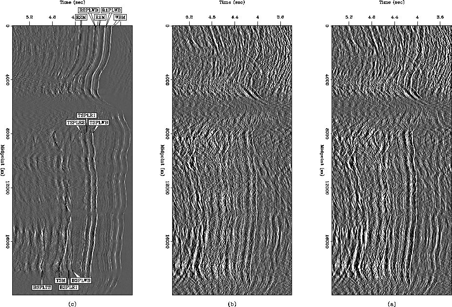
Finally, Figure ![[*]](http://sepwww.stanford.edu/latex2html/cross_ref_motif.gif) shows the stack of the LSJIMP
estimated primaries after the nonlinear update. The Figure is directly
comparable with Figure
shows the stack of the LSJIMP
estimated primaries after the nonlinear update. The Figure is directly
comparable with Figure ![[*]](http://sepwww.stanford.edu/latex2html/cross_ref_motif.gif) . Again, the differences are
quite subtle. Notice an improvement in the removal of deep, salt-related
multiple events, like BSPLTS.
. Again, the differences are
quite subtle. Notice an improvement in the removal of deep, salt-related
multiple events, like BSPLTS.
stackcomp-iter1.gulf
Figure 32
Top: raw data stack. Center: estimated LSJIMP primaries stack after nonlinear
updating of crosstalk weights and reflection coefficients. Bottom: difference
panel (estimated multiples) stack. Figure annotated and displayed with same
gain and clip as Figure ![[*]](http://sepwww.stanford.edu/latex2html/cross_ref_motif.gif) .
.
![[*]](http://sepwww.stanford.edu/latex2html/movie.gif)


Next: 3-D Theory \label>chapter:theory3d>
Up: 2-D Field Data Results
Previous: Playing Devil's Advocate: What
Stanford Exploration Project
5/30/2004
![[*]](http://sepwww.stanford.edu/latex2html/cross_ref_motif.gif) on the Mississippi Canyon data. I ran only one
nonlinear iteration. Since the velocity model is already quite nicely
determined, I did not do residual velocity analysis after the first run of
LSJIMP. However, I did recompute the crosstalk weights and the reflection
coefficients for each of the four multiple generators.
on the Mississippi Canyon data. I ran only one
nonlinear iteration. Since the velocity model is already quite nicely
determined, I did not do residual velocity analysis after the first run of
LSJIMP. However, I did recompute the crosstalk weights and the reflection
coefficients for each of the four multiple generators.

![[*]](http://sepwww.stanford.edu/latex2html/movie.gif)


