

Next: Nonlinear Iteration Test
Up: 2-D Field Data Results
Previous: SRME versus HEMNO
LSJIMP seeks to exploit another type of multiplicity in the data, that between
multiples and primaries. I claimed in Chapter ![[*]](http://sepwww.stanford.edu/latex2html/cross_ref_motif.gif) that by
adding the model regularization which differences between images (section
that by
adding the model regularization which differences between images (section
![[*]](http://sepwww.stanford.edu/latex2html/cross_ref_motif.gif) ), we expect that information from the multiples can fill
illumination holes or missing trace and also lead to better discrimination
between signal and noise. The veracity of this claim is central to the labeling
of LSJIMP as a ``joint imaging'' algorithm. If false, then we conclude that the
multiples add nothing to the inversion. I ran a simple test to determine what,
if anything, the multiples add to the LSJIMP inversion, I ``turn off'' the
regularization which differences across images by setting
), we expect that information from the multiples can fill
illumination holes or missing trace and also lead to better discrimination
between signal and noise. The veracity of this claim is central to the labeling
of LSJIMP as a ``joint imaging'' algorithm. If false, then we conclude that the
multiples add nothing to the inversion. I ran a simple test to determine what,
if anything, the multiples add to the LSJIMP inversion, I ``turn off'' the
regularization which differences across images by setting  in
equation (
in
equation (![[*]](http://sepwww.stanford.edu/latex2html/cross_ref_motif.gif) ). Figures
). Figures
![[*]](http://sepwww.stanford.edu/latex2html/cross_ref_motif.gif) -
-![[*]](http://sepwww.stanford.edu/latex2html/cross_ref_motif.gif) show the results of this
test.
show the results of this
test.
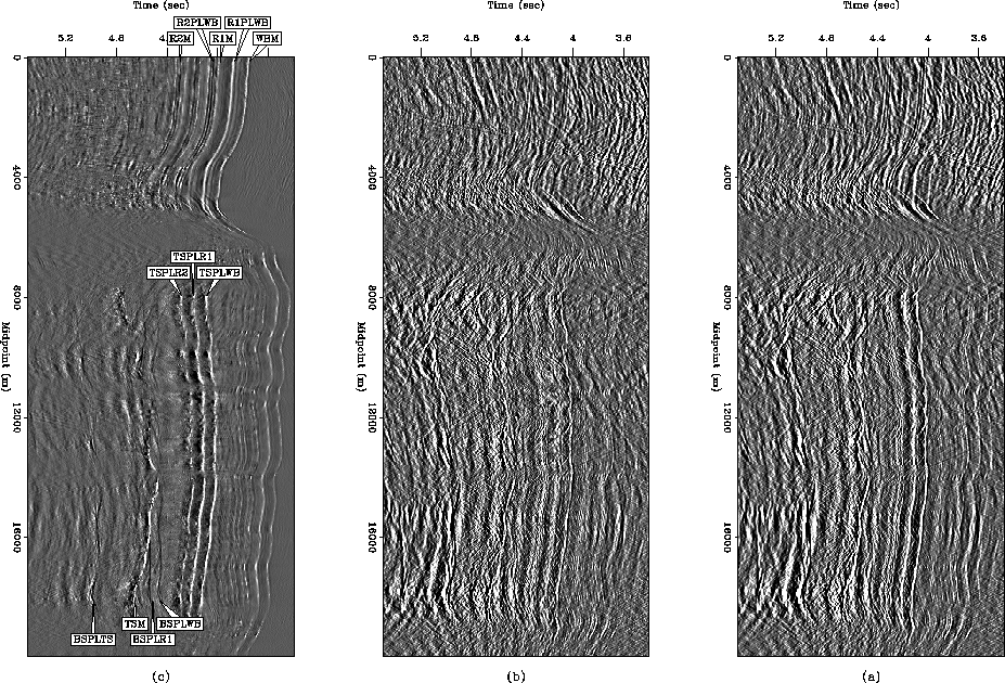
Figure ![[*]](http://sepwww.stanford.edu/latex2html/cross_ref_motif.gif) shows the stack of the estimated
primaries,
shows the stack of the estimated
primaries,  , with
  , and can be compared directly with
Figure
 ![[*]](http://sepwww.stanford.edu/latex2html/cross_ref_motif.gif) . Differences are apparent, although subtle.
Generally, we notice a loss of coherency in the estimated multiples (difference
panel).
. Differences are apparent, although subtle.
Generally, we notice a loss of coherency in the estimated multiples (difference
panel).
stackcomp-devils.gulf
Figure 25
Top: raw data stack. Center: estimated LSJIMP primaries stack, with
 . Bottom: difference panel (estimated multiples) stack.
Compare with Figure
 ![[*]](http://sepwww.stanford.edu/latex2html/cross_ref_motif.gif) .
.
![[*]](http://sepwww.stanford.edu/latex2html/movie.gif)


More revealing are Figures ![[*]](http://sepwww.stanford.edu/latex2html/cross_ref_motif.gif) and
and
![[*]](http://sepwww.stanford.edu/latex2html/cross_ref_motif.gif) , which show a zoomed view of two regions
of Figure
, which show a zoomed view of two regions
of Figure ![[*]](http://sepwww.stanford.edu/latex2html/cross_ref_motif.gif) , and are directly comparable to
Figures
, and are directly comparable to
Figures ![[*]](http://sepwww.stanford.edu/latex2html/cross_ref_motif.gif) and
and ![[*]](http://sepwww.stanford.edu/latex2html/cross_ref_motif.gif) ,
respectively. Comparing Figure
,
respectively. Comparing Figure ![[*]](http://sepwww.stanford.edu/latex2html/cross_ref_motif.gif) to
Figure
to
Figure ![[*]](http://sepwww.stanford.edu/latex2html/cross_ref_motif.gif) , we again note a general decrease in
estimated multiple coherency when
, we again note a general decrease in
estimated multiple coherency when  . We also can see that in
regions where multiples overlap primaries, like at 3.7 seconds/1200 meters,
setting
  leads to some losses in primary energy. Comparing
Figure
 ![[*]](http://sepwww.stanford.edu/latex2html/cross_ref_motif.gif) to Figure
to Figure
![[*]](http://sepwww.stanford.edu/latex2html/cross_ref_motif.gif) , we see that setting
, we see that setting  leads to a
generally worse result. Less multiple energy is removed, particularly from some
of the salt-related multiples, like TSPLWB and BSPLWB, and again, the subtracted
energy is less coherent.
stackcomp-devils.zoom.1.gulf
Figure 26
Zoom on Figure ![[*]](http://sepwww.stanford.edu/latex2html/cross_ref_motif.gif) , from the sedimentary basin
section of the data. Top: raw data stack. Center: estimated LSJIMP primaries
stack, with
, from the sedimentary basin
section of the data. Top: raw data stack. Center: estimated LSJIMP primaries
stack, with  . Bottom: difference panel (estimated multiples)
stack. Compare with Figure
 ![[*]](http://sepwww.stanford.edu/latex2html/cross_ref_motif.gif) .
.
![[*]](http://sepwww.stanford.edu/latex2html/movie.gif)


stackcomp-devils.zoom.3.gulf
Figure 27
Zoom on Figure ![[*]](http://sepwww.stanford.edu/latex2html/cross_ref_motif.gif) , from the subsalt section of
the data. Top: raw data stack. Center: estimated LSJIMP primaries stack,
with
, from the subsalt section of
the data. Top: raw data stack. Center: estimated LSJIMP primaries stack,
with  . Bottom: difference panel (estimated multiples) stack.
Compare with Figure
 ![[*]](http://sepwww.stanford.edu/latex2html/cross_ref_motif.gif) .
.
![[*]](http://sepwww.stanford.edu/latex2html/movie.gif)


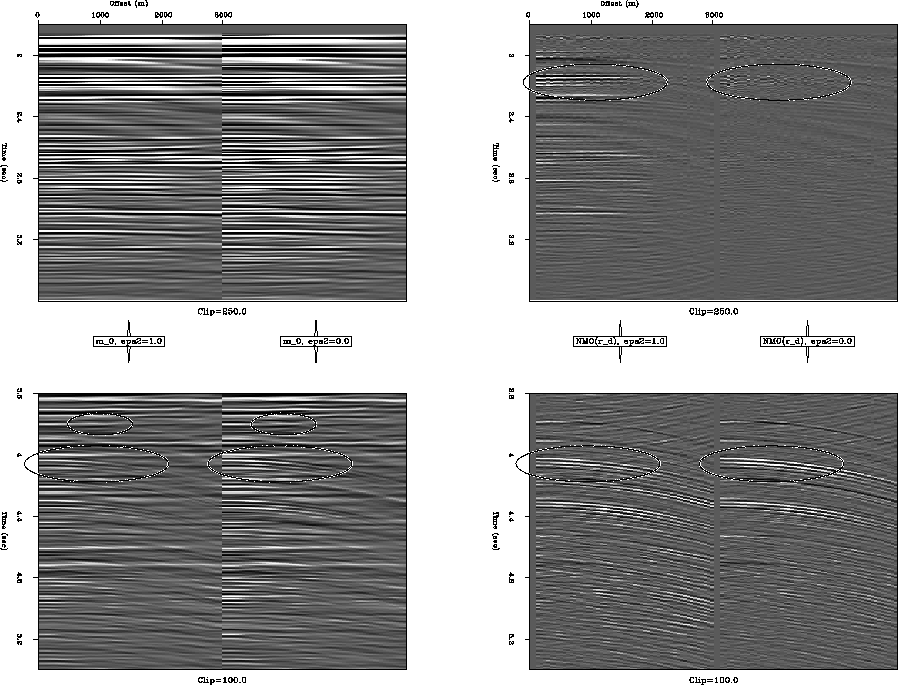
Finally, Figure ![[*]](http://sepwww.stanford.edu/latex2html/cross_ref_motif.gif) compares the result of setting
compares the result of setting
 in the prestack sense, at CMP 55 of 750. The left-hand panels
compare the estimated primaries with
  and
and  , while
the right-hand panels compare (after NMO) the data residuals for
 and
and  . The panels are split in half vertically
and clipped at a different value, labeled on the plot, for display purposes.
Comparing the estimated primaries, we see from the small oval that where
multiples and primaries overlap, setting
  reduces the quality of
the separation. Primaries are less coherent with offset, and the primary
panel contains some energy corresponding to the seabed pure multiple. From the
larger oval, notice that for the strongest multiples, setting
  leads to poorer separation. Comparing the data residuals, we see from the top
pair of ovals that if
  , we generally somewhat damage the
primaries, which we expect if we have velocity errors, mis-alignment between
imaged primaries and multiples, or incorrect reflection coefficient. This issue
was discussed earlier, in section
 ![[*]](http://sepwww.stanford.edu/latex2html/cross_ref_motif.gif) . However, we also
note from the lower pair of ovals, that setting
. However, we also
note from the lower pair of ovals, that setting  seems to have
reduced our ability to accurately model the important multiples.
devils.gulf
Figure 28
Left-hand panels: Estimated LSJIMP primaries at CMP 55 of 750, with
 and
and  . Right-hand panels: Weighted data
residuals at CMP 55 (after NMO) with
  and
and  . Left-hand and right-hand panels split in half along time axis and clipped
independently for display clarity.
![[*]](http://sepwww.stanford.edu/latex2html/movie.gif)


Next: Nonlinear Iteration Test
Up: 2-D Field Data Results
Previous: SRME versus HEMNO
Stanford Exploration Project
5/30/2004
![[*]](http://sepwww.stanford.edu/latex2html/cross_ref_motif.gif) that by
adding the model regularization which differences between images (section
that by
adding the model regularization which differences between images (section
![[*]](http://sepwww.stanford.edu/latex2html/cross_ref_motif.gif) ), we expect that information from the multiples can fill
illumination holes or missing trace and also lead to better discrimination
between signal and noise. The veracity of this claim is central to the labeling
of LSJIMP as a ``joint imaging'' algorithm. If false, then we conclude that the
multiples add nothing to the inversion. I ran a simple test to determine what,
if anything, the multiples add to the LSJIMP inversion, I ``turn off'' the
regularization which differences across images by setting
), we expect that information from the multiples can fill
illumination holes or missing trace and also lead to better discrimination
between signal and noise. The veracity of this claim is central to the labeling
of LSJIMP as a ``joint imaging'' algorithm. If false, then we conclude that the
multiples add nothing to the inversion. I ran a simple test to determine what,
if anything, the multiples add to the LSJIMP inversion, I ``turn off'' the
regularization which differences across images by setting ![[*]](http://sepwww.stanford.edu/latex2html/cross_ref_motif.gif) ). Figures
). Figures
![[*]](http://sepwww.stanford.edu/latex2html/cross_ref_motif.gif) -
-![[*]](http://sepwww.stanford.edu/latex2html/cross_ref_motif.gif) show the results of this
test.
show the results of this
test.

![[*]](http://sepwww.stanford.edu/latex2html/movie.gif)


