![[*]](http://sepwww.stanford.edu/latex2html/cross_ref_motif.gif) , the data contain a variety of strong surface-related
multiples which hamper primary imaging, and enough geologic complexity to render
one-dimensional multiple suppression methods ineffectual.
, the data contain a variety of strong surface-related
multiples which hamper primary imaging, and enough geologic complexity to render
one-dimensional multiple suppression methods ineffectual.
In 1997, WesternGeco distributed a 2-D dataset, acquired in the Mississippi
Canyon region of the Gulf of Mexico, for the testing of multiple suppression
algorithms. As illustrated on the CMP-stacked section, Figure
![[*]](http://sepwww.stanford.edu/latex2html/cross_ref_motif.gif) , the data contain a variety of strong surface-related
multiples which hamper primary imaging, and enough geologic complexity to render
one-dimensional multiple suppression methods ineffectual.
, the data contain a variety of strong surface-related
multiples which hamper primary imaging, and enough geologic complexity to render
one-dimensional multiple suppression methods ineffectual.
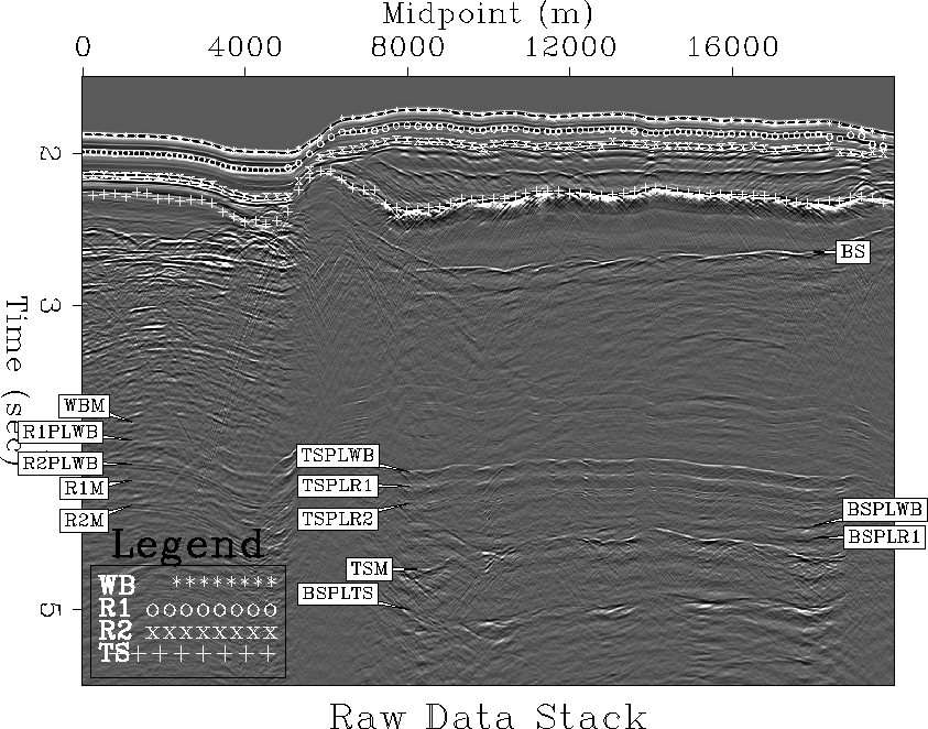 |
In this chapter, I show the results of testing my particular implementation of
the LSJIMP technique on 750 CMP locations of the Mississippi Canyon dataset,
modeling four multiple generators-the seabed, two strong shallow reflectors,
and the top of salt-as labeled by the picks on Figure ![[*]](http://sepwww.stanford.edu/latex2html/cross_ref_motif.gif) .
Only first order multiples are included in the inversion. Thus in equation
(
.
Only first order multiples are included in the inversion. Thus in equation
(![[*]](http://sepwww.stanford.edu/latex2html/cross_ref_motif.gif) ),
), ![]() and p=1.
and p=1.
Estimation of a multiple generator's reflection coefficient is a crucially
important step in my implementation of LSJIMP. Figures
![[*]](http://sepwww.stanford.edu/latex2html/cross_ref_motif.gif) -
-![[*]](http://sepwww.stanford.edu/latex2html/cross_ref_motif.gif) illustrate the result of applying the
reflection coefficient methodology outlined in Section
illustrate the result of applying the
reflection coefficient methodology outlined in Section ![[*]](http://sepwww.stanford.edu/latex2html/cross_ref_motif.gif) to each
of the four multiple generators shown in Figure
to each
of the four multiple generators shown in Figure ![[*]](http://sepwww.stanford.edu/latex2html/cross_ref_motif.gif) . Each
Figure shows a stack of the local windows around the primary reflection and first
pure multiple after alignment with cross-correlation, weighted by a user-defined
residual weight which is set to zero where the data appear incoherent, and to one
elsewhere. The seabed and R1 reflections (Figures
. Each
Figure shows a stack of the local windows around the primary reflection and first
pure multiple after alignment with cross-correlation, weighted by a user-defined
residual weight which is set to zero where the data appear incoherent, and to one
elsewhere. The seabed and R1 reflections (Figures ![[*]](http://sepwww.stanford.edu/latex2html/cross_ref_motif.gif) and
and
![[*]](http://sepwww.stanford.edu/latex2html/cross_ref_motif.gif) ) have the greatest coherency, with fairly consistent
estimated reflection coefficients across all midpoints, although the R1 pure
multiple partially overlaps the strong R2 seabed pegleg and tends to bias the
estimated R1 reflection coefficient upward. The short wavelength of the
multi-peaked R2 reflection (Figure
) have the greatest coherency, with fairly consistent
estimated reflection coefficients across all midpoints, although the R1 pure
multiple partially overlaps the strong R2 seabed pegleg and tends to bias the
estimated R1 reflection coefficient upward. The short wavelength of the
multi-peaked R2 reflection (Figure ![[*]](http://sepwww.stanford.edu/latex2html/cross_ref_motif.gif) ) cause offset-dependent
tuning effects that somewhat degrades our ability to reliably estimate a
reflection coefficient. Lastly, strong head waves and a rugose salt top degrade
the coherency of the top-of-salt reflection and its multiple (Figure
) cause offset-dependent
tuning effects that somewhat degrades our ability to reliably estimate a
reflection coefficient. Lastly, strong head waves and a rugose salt top degrade
the coherency of the top-of-salt reflection and its multiple (Figure
![[*]](http://sepwww.stanford.edu/latex2html/cross_ref_motif.gif) ), although we can get a fairly reliable estimate between
midpoints of about 12000 and 18000 meters.
), although we can get a fairly reliable estimate between
midpoints of about 12000 and 18000 meters.
|
rc.1.gulf
Figure 2 Top: Stack of window around seabed reflection (WB). Center: Stack of window around seabed pure multiple (WBM). Bottom: estimated WB reflection coefficient. | 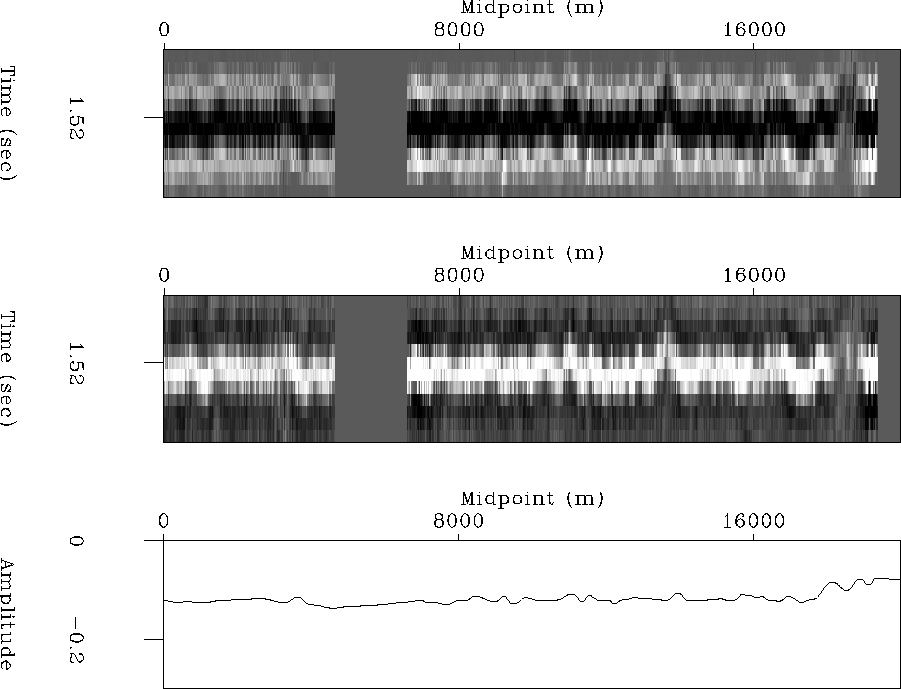 |
|
rc.2.gulf
Figure 3 Top: Stack of window around R1 reflection. Center: Stack of window around R1 pure multiple (R1M). Bottom: estimated R1 reflection coefficient. | 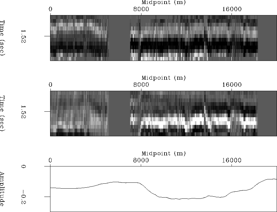 |
|
rc.3.gulf
Figure 4 Top: Stack of window around R2 reflection. Center: Stack of window around R2 pure multiple (R2M). Bottom: estimated R2 reflection coefficient. | 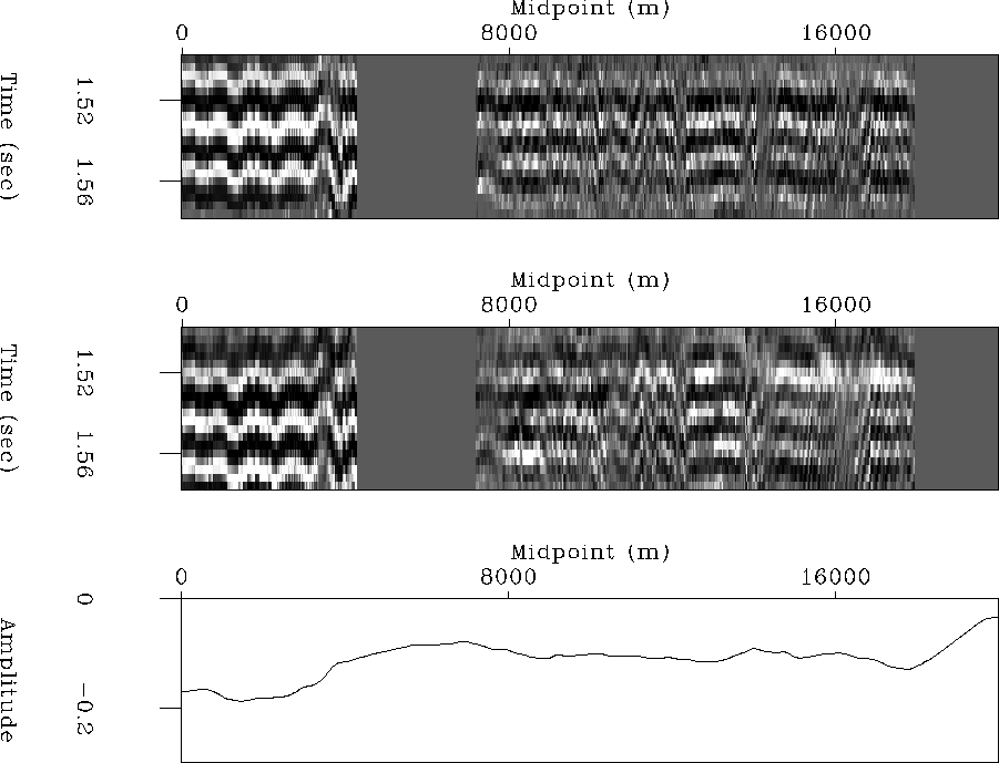 |
|
rc.4.gulf
Figure 5 Top: Stack of window around top-of-salt reflection (TS). Center: Stack of window around top-of-salt pure multiple (TSM). Bottom: estimated TS reflection coefficient. | 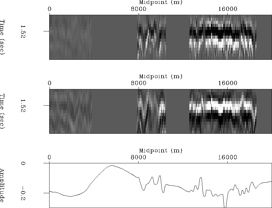 |
WesternGeco supplied a depth interval velocity model, so computation of stacking
velocities was trivial. I ran LSJIMP with 20 conjugate gradient iterations on 28
CPUs (1.3 Ghz Pentium 3) of a Linux cluster, for a total run time of around 3
hours, including all I/O. Coincidentally, the run time is very similar to the
prestack wave-equation depth migration run to generate the results in section
![[*]](http://sepwww.stanford.edu/latex2html/cross_ref_motif.gif) .
.
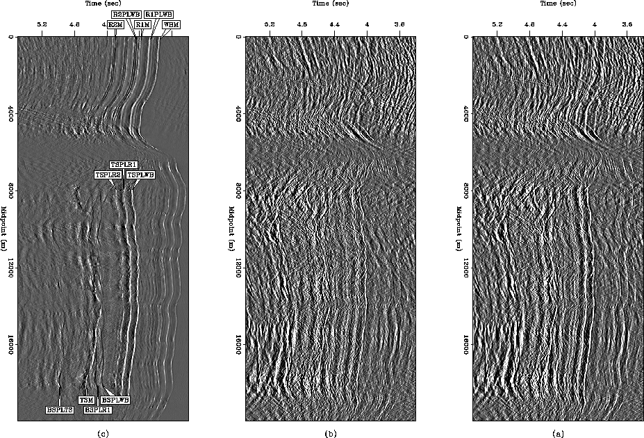
Figure ![[*]](http://sepwww.stanford.edu/latex2html/cross_ref_motif.gif) illustrates the stack of the LSJIMP primary
image,
illustrates the stack of the LSJIMP primary
image, ![]() , which should contain only primaries. From the difference
panel (c), note that important above-salt peglegs are almost entirely removed.
Primaries are not visibly damaged. Salt rugosity contributes negatively to the
separation, by forming diffractions that are not modeled by HEMNO, and by
violating HEMNO's small reflector dip assumption. Still, LSJIMP does a fairly
good job of removing the specular components of strong salt-related multiples.
Some deep multiple energy remains. While unmodeled multiple events, such as
internal salt multiples, may explain the residual, another likely contributor is
the complex subsalt wave propagation. Time imaging operators like HEMNO
generally perform more poorly than depth migration below large velocity
contrasts.
, which should contain only primaries. From the difference
panel (c), note that important above-salt peglegs are almost entirely removed.
Primaries are not visibly damaged. Salt rugosity contributes negatively to the
separation, by forming diffractions that are not modeled by HEMNO, and by
violating HEMNO's small reflector dip assumption. Still, LSJIMP does a fairly
good job of removing the specular components of strong salt-related multiples.
Some deep multiple energy remains. While unmodeled multiple events, such as
internal salt multiples, may explain the residual, another likely contributor is
the complex subsalt wave propagation. Time imaging operators like HEMNO
generally perform more poorly than depth migration below large velocity
contrasts.
 |
![[*]](http://sepwww.stanford.edu/latex2html/cross_ref_motif.gif) .
.
Figures ![[*]](http://sepwww.stanford.edu/latex2html/cross_ref_motif.gif) and
and ![[*]](http://sepwww.stanford.edu/latex2html/cross_ref_motif.gif) make
the same comparison as Figure
make
the same comparison as Figure ![[*]](http://sepwww.stanford.edu/latex2html/cross_ref_motif.gif) , but in small windows to
emphasize local features. The geological context of Figure
, but in small windows to
emphasize local features. The geological context of Figure
![[*]](http://sepwww.stanford.edu/latex2html/cross_ref_motif.gif) is a generally well-behaved sedimentary basin,
with shallow dips and low velocity contrast. Notice that a variety of strong
peglegs are largely removed without badly damaging the many updipping primary
events in the section. Figure
is a generally well-behaved sedimentary basin,
with shallow dips and low velocity contrast. Notice that a variety of strong
peglegs are largely removed without badly damaging the many updipping primary
events in the section. Figure ![[*]](http://sepwww.stanford.edu/latex2html/cross_ref_motif.gif) is taken from
over the tabular salt body. The multiples visible in this window are effectively
separated from the data, even those from the top and bottom of the salt. Weak
subsalt primaries, like the anticlinal structure which peaks around CMP 16000 m
are not visibly harmed by the separation.
is taken from
over the tabular salt body. The multiples visible in this window are effectively
separated from the data, even those from the top and bottom of the salt. Weak
subsalt primaries, like the anticlinal structure which peaks around CMP 16000 m
are not visibly harmed by the separation.
 |
![[*]](http://sepwww.stanford.edu/latex2html/cross_ref_motif.gif) .
.
 |
![[*]](http://sepwww.stanford.edu/latex2html/cross_ref_motif.gif) . Subsalt primary events labeled ``P''.
. Subsalt primary events labeled ``P''.
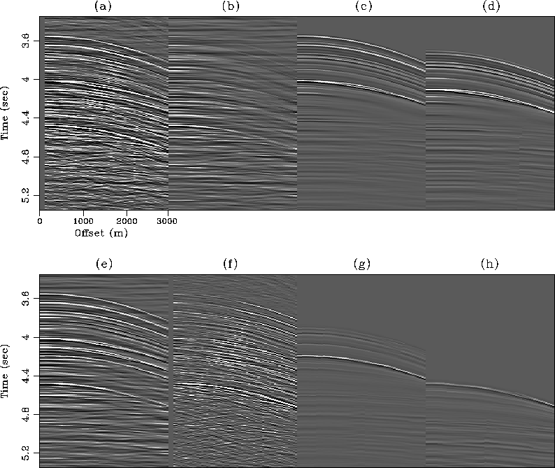
Figures ![[*]](http://sepwww.stanford.edu/latex2html/cross_ref_motif.gif) -
-![[*]](http://sepwww.stanford.edu/latex2html/cross_ref_motif.gif) show the
LSJIMP results at three midpoint locations. In each Figure, panels (c), (d),
(g), and (h) illustrate the estimated total first order multiple from each of the
four multiple generators. For instance, to generate the estimated seabed pegleg
panel (c), we construct a model vector,
show the
LSJIMP results at three midpoint locations. In each Figure, panels (c), (d),
(g), and (h) illustrate the estimated total first order multiple from each of the
four multiple generators. For instance, to generate the estimated seabed pegleg
panel (c), we construct a model vector,
| |
(29) |
| |
(30) |
Figure ![[*]](http://sepwww.stanford.edu/latex2html/cross_ref_motif.gif) comes from the sedimentary basin portion
of the data. The multiples on this gather have fairly simple moveout behavior.
From the relatively small amount of correlated energy on the residual error panel
(f), we see that most multiples present in the data are modeled well by LSJIMP.
However, notice the introduction of a ``new'' event to the modeled data around
comes from the sedimentary basin portion
of the data. The multiples on this gather have fairly simple moveout behavior.
From the relatively small amount of correlated energy on the residual error panel
(f), we see that most multiples present in the data are modeled well by LSJIMP.
However, notice the introduction of a ``new'' event to the modeled data around
![]() . The R1M event overlaps with R2PLWB, which leads to crosstalk
leakage and a poor estimate of R1's reflection coefficient. As we will see
later, in section
. The R1M event overlaps with R2PLWB, which leads to crosstalk
leakage and a poor estimate of R1's reflection coefficient. As we will see
later, in section ![[*]](http://sepwww.stanford.edu/latex2html/cross_ref_motif.gif) , the nonlinear updating scheme of
section
, the nonlinear updating scheme of
section ![[*]](http://sepwww.stanford.edu/latex2html/cross_ref_motif.gif) helps solve this problem.
helps solve this problem.
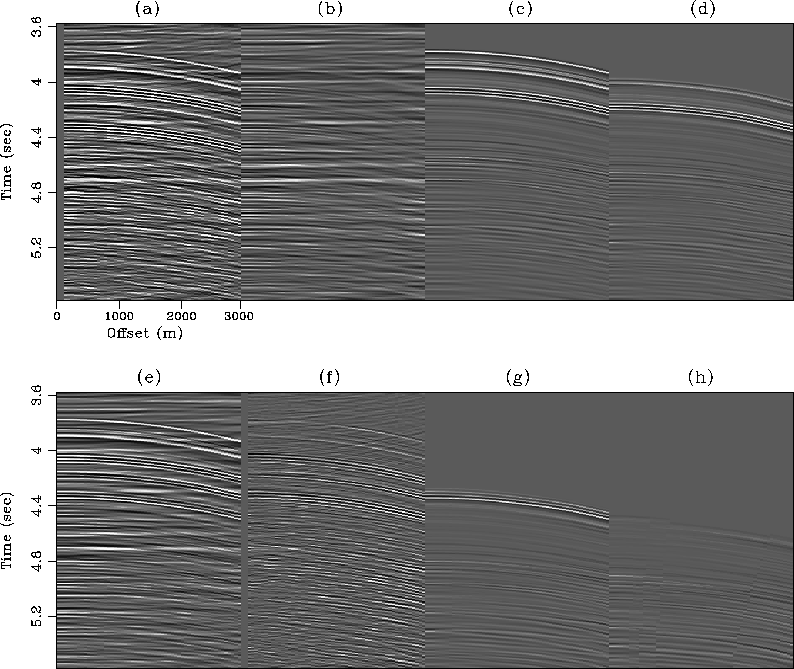 |
![[*]](http://sepwww.stanford.edu/latex2html/cross_ref_motif.gif) . All panels NMO'ed with stacking velocity and
windowed in time from 3.5 to 5.5 seconds and gained with t2. (a) Raw data;
(b) Estimated primaries (
. All panels NMO'ed with stacking velocity and
windowed in time from 3.5 to 5.5 seconds and gained with t2. (a) Raw data;
(b) Estimated primaries (
Figure ![[*]](http://sepwww.stanford.edu/latex2html/cross_ref_motif.gif) is drawn from the left-hand side of the
salt body. The separation results are quite good, both for the relatively simple
shallow multiples and for the complex salt-related multiples, which visibly
split. A flat event around 4.5 seconds, which appears to be a primary, is
actually most likely a pegleg multiple from the base of salt, flattened because
the stacking velocity decreases below the salt.
is drawn from the left-hand side of the
salt body. The separation results are quite good, both for the relatively simple
shallow multiples and for the complex salt-related multiples, which visibly
split. A flat event around 4.5 seconds, which appears to be a primary, is
actually most likely a pegleg multiple from the base of salt, flattened because
the stacking velocity decreases below the salt.
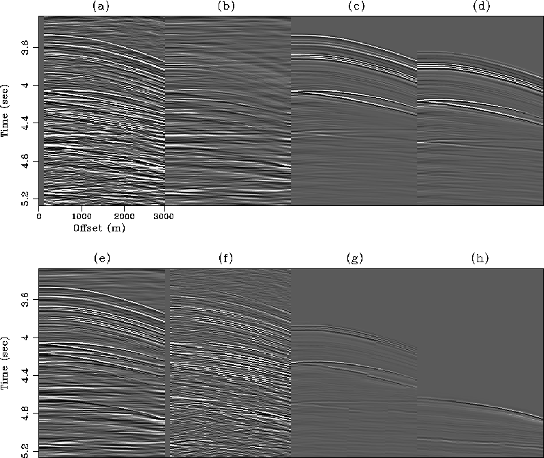 |
![[*]](http://sepwww.stanford.edu/latex2html/cross_ref_motif.gif) . All panels NMO'ed with stacking velocity and
windowed in time from 3.5 to 5.5 seconds and gained with t2. (a) Raw data;
(b) Estimated primaries (
. All panels NMO'ed with stacking velocity and
windowed in time from 3.5 to 5.5 seconds and gained with t2. (a) Raw data;
(b) Estimated primaries (
Figure ![[*]](http://sepwww.stanford.edu/latex2html/cross_ref_motif.gif) is drawn from the right-hand side of the
salt body. As with Figure
is drawn from the right-hand side of the
salt body. As with Figure ![[*]](http://sepwww.stanford.edu/latex2html/cross_ref_motif.gif) , some of the complex
splitting behavior in the salt-related peglegs is effectively modeled by HEMNO.
In this case, the reflector dips are such that the events split at medium
offsets, but happen to coincide at far offsets. Signal events are quite
difficult to spot under the multiples, but some shallow events are uncovered.
, some of the complex
splitting behavior in the salt-related peglegs is effectively modeled by HEMNO.
In this case, the reflector dips are such that the events split at medium
offsets, but happen to coincide at far offsets. Signal events are quite
difficult to spot under the multiples, but some shallow events are uncovered.
 |
![[*]](http://sepwww.stanford.edu/latex2html/cross_ref_motif.gif) . All panels NMO'ed with stacking velocity and
windowed in time from 3.5 to 5.5 seconds and gained with t2. (a) Raw data;
(b) Estimated primaries (
. All panels NMO'ed with stacking velocity and
windowed in time from 3.5 to 5.5 seconds and gained with t2. (a) Raw data;
(b) Estimated primaries (