

Next: SRME versus HEMNO
Up: 2-D Field Data Results
Previous: Depth Migration Before and
The theoretical development of the LSJIMP algorithm given in Chapter
![[*]](http://sepwww.stanford.edu/latex2html/cross_ref_motif.gif) defines the data and model residuals in mathematical and
algorithmic terms, but in this section, I more practically illustrate the
structure of and relationship between the residual vectors with a real data
example. Figures
defines the data and model residuals in mathematical and
algorithmic terms, but in this section, I more practically illustrate the
structure of and relationship between the residual vectors with a real data
example. Figures ![[*]](http://sepwww.stanford.edu/latex2html/cross_ref_motif.gif) -
-![[*]](http://sepwww.stanford.edu/latex2html/cross_ref_motif.gif) were computed
at CMP 55 or 750 of the Mississippi Canyon 2-D dataset, in the sedimentary
region of the data. Figures which display seismic data are divided in half along
the time axis and clipped independently for viewing purposes.
were computed
at CMP 55 or 750 of the Mississippi Canyon 2-D dataset, in the sedimentary
region of the data. Figures which display seismic data are divided in half along
the time axis and clipped independently for viewing purposes.
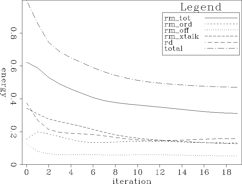
Figure ![[*]](http://sepwww.stanford.edu/latex2html/cross_ref_motif.gif) illustrates, as a function of conjugate gradient
iteration, the norm of the data and model residuals from the LSJIMP inversion at
CMP 55. Although the norm of the combined model and data residual [equation
(
illustrates, as a function of conjugate gradient
iteration, the norm of the data and model residuals from the LSJIMP inversion at
CMP 55. Although the norm of the combined model and data residual [equation
(![[*]](http://sepwww.stanford.edu/latex2html/cross_ref_motif.gif) )] is guaranteed to decrease with iteration, we see that the
individual residuals may decrease at different rates, or even increase with
iteration. Of particular interest in the Figure is the model residual
corresponding to differentiation across individual images (
)] is guaranteed to decrease with iteration, we see that the
individual residuals may decrease at different rates, or even increase with
iteration. Of particular interest in the Figure is the model residual
corresponding to differentiation across individual images (![$\bold r_m^{[1]}$](img122.gif) in
equation (
in
equation (![[*]](http://sepwww.stanford.edu/latex2html/cross_ref_motif.gif) )). As a starting guess, I simply ``spread'' a
stacked trace of the primaries across all offsets, for all images.
)). As a starting guess, I simply ``spread'' a
stacked trace of the primaries across all offsets, for all images.
![$\bold r_m^{[1]}$](img122.gif) is roughly a measure of image dissimilarity. As the images are
adjusted to fit variations in the data, the images become more dissimilar, and
the model residual initially increases, before decreasing slowly with iteration.
is roughly a measure of image dissimilarity. As the images are
adjusted to fit variations in the data, the images become more dissimilar, and
the model residual initially increases, before decreasing slowly with iteration.


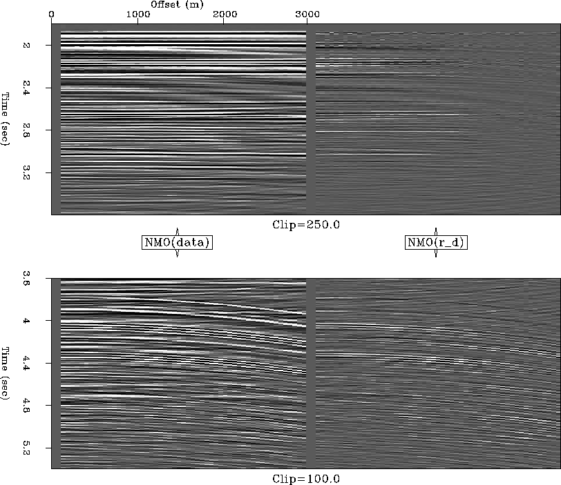
Figure ![[*]](http://sepwww.stanford.edu/latex2html/cross_ref_motif.gif) compares the data residual and raw data at CMP 55.
A somewhat similar comparison was made earlier, in Figures
compares the data residual and raw data at CMP 55.
A somewhat similar comparison was made earlier, in Figures
![[*]](http://sepwww.stanford.edu/latex2html/cross_ref_motif.gif) -
-![[*]](http://sepwww.stanford.edu/latex2html/cross_ref_motif.gif) , to examine the
quality of fit to the multiples, but the earlier portions of the time axis were
not shown. At earlier times, notice that the data residual contains some primary
energy. The model regularization terms in the LSJIMP inversion cause the misfit.
LSJIMP's working definition of ``signal'' includes events that are perfectly flat
with offset on all images (with ``smooth'' AVO variation) and perfectly
self-consistent multiple and primary images. If, for instance, the stacking
velocity does not perfectly flatten a primary, or if primary and multiple events
are misaligned or mis-modeled in terms of amplitude, we will see some primary
energy in the data residual. Furthermore, notice increased misfit at near
offsets versus far offsets. As noted in Section
, to examine the
quality of fit to the multiples, but the earlier portions of the time axis were
not shown. At earlier times, notice that the data residual contains some primary
energy. The model regularization terms in the LSJIMP inversion cause the misfit.
LSJIMP's working definition of ``signal'' includes events that are perfectly flat
with offset on all images (with ``smooth'' AVO variation) and perfectly
self-consistent multiple and primary images. If, for instance, the stacking
velocity does not perfectly flatten a primary, or if primary and multiple events
are misaligned or mis-modeled in terms of amplitude, we will see some primary
energy in the data residual. Furthermore, notice increased misfit at near
offsets versus far offsets. As noted in Section ![[*]](http://sepwww.stanford.edu/latex2html/cross_ref_motif.gif) , the
model regularization operators are not applied where the multiples provide no
information - specifically, as far offsets, as dictated by Snell Resmpling. The
fact that we see little to no residual primary energy at far offsets confirms the
notion that model regularization terms cause the observed misfit at near offsets.
, the
model regularization operators are not applied where the multiples provide no
information - specifically, as far offsets, as dictated by Snell Resmpling. The
fact that we see little to no residual primary energy at far offsets confirms the
notion that model regularization terms cause the observed misfit at near offsets.
resd.gulf
Figure 16
Raw data (left) and data residual (right) compared for CMP 55 of 750. NMO
with primary stacking velocity applied to facilitate discrimination between
multiples and primaries.


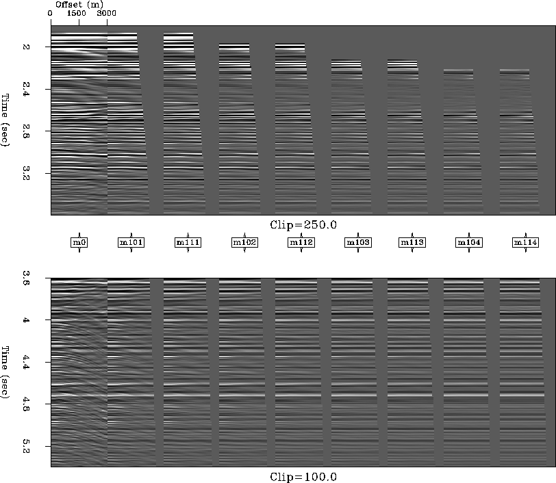
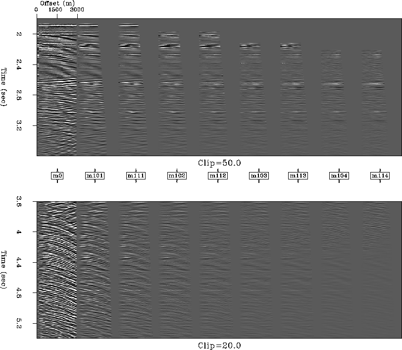
Figure ![[*]](http://sepwww.stanford.edu/latex2html/cross_ref_motif.gif) simply shows all nine (four multiple generators,
first-order multiples only) panels of the model space at CMP 55. Comparing the
primary image (''m0'') directly with the raw data shown in Figure
simply shows all nine (four multiple generators,
first-order multiples only) panels of the model space at CMP 55. Comparing the
primary image (''m0'') directly with the raw data shown in Figure
![[*]](http://sepwww.stanford.edu/latex2html/cross_ref_motif.gif) , notice that obvious multiples have been strongly, but not
totally, suppressed and that two prominent primary reflections between 4.4 and
4.8 seconds uncovered. This Figure and Figures
, notice that obvious multiples have been strongly, but not
totally, suppressed and that two prominent primary reflections between 4.4 and
4.8 seconds uncovered. This Figure and Figures
![[*]](http://sepwww.stanford.edu/latex2html/cross_ref_motif.gif) -
-![[*]](http://sepwww.stanford.edu/latex2html/cross_ref_motif.gif) , which display the various
model residual vectors, have the same graphical layout.
, which display the various
model residual vectors, have the same graphical layout.
model.gulf
Figure 17
LSJIMP model space at CMP 55 of 750. ``m0'' is the primary image,
 , while ``mikm'' corresponds to
  , the image of the
 split of the
  -order pegleg multiple from the
 multiple generator.


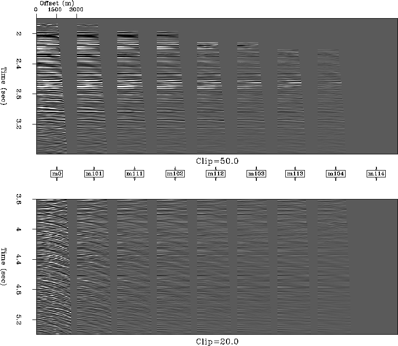
Figure ![[*]](http://sepwww.stanford.edu/latex2html/cross_ref_motif.gif) illustrates the model residual corresponding to
the differencing across images regularization operator derived in Section
illustrates the model residual corresponding to
the differencing across images regularization operator derived in Section
![[*]](http://sepwww.stanford.edu/latex2html/cross_ref_motif.gif) , and to
, and to ![$\bold r_m^{[1]}$](img122.gif) in equation (
in equation (![[*]](http://sepwww.stanford.edu/latex2html/cross_ref_motif.gif) ).
First notice that the last panel, ``m114'' is blank. The differencing operator
subtracts one image panel from the previous, in exactly the left-to-right order
shown on the Figure. The difference is not defined for the last image, here
``m114''. The difference is zero-valued at far offsets, because the multiples
provide no information here, as mentioned in the discussion of Figure
).
First notice that the last panel, ``m114'' is blank. The differencing operator
subtracts one image panel from the previous, in exactly the left-to-right order
shown on the Figure. The difference is not defined for the last image, here
``m114''. The difference is zero-valued at far offsets, because the multiples
provide no information here, as mentioned in the discussion of Figure
![[*]](http://sepwww.stanford.edu/latex2html/cross_ref_motif.gif) . Above the onset of the seabed pure multiple, notice on the
residual panels some primary energy, the presence of which can be explained by
misalignment of primaries and multiples after imaging or by inaccuracies in the
amplitude modeling of the multiples. In theory, after proper imaging, the
multiples should be ``copies of the primary''; any deviations from this state
will appear on the model residual shown in Figure
. Above the onset of the seabed pure multiple, notice on the
residual panels some primary energy, the presence of which can be explained by
misalignment of primaries and multiples after imaging or by inaccuracies in the
amplitude modeling of the multiples. In theory, after proper imaging, the
multiples should be ``copies of the primary''; any deviations from this state
will appear on the model residual shown in Figure ![[*]](http://sepwww.stanford.edu/latex2html/cross_ref_motif.gif) . At
later times, we notice considerable residual multiple energy. As discussed in
Section
. At
later times, we notice considerable residual multiple energy. As discussed in
Section ![[*]](http://sepwww.stanford.edu/latex2html/cross_ref_motif.gif) (Figure
(Figure ![[*]](http://sepwww.stanford.edu/latex2html/cross_ref_motif.gif) ), crosstalk events
from one image panel to another do not generally coincide at far offsets.
), crosstalk events
from one image panel to another do not generally coincide at far offsets.
resm.order.gulf
Figure 18
LSJIMP model residual ![$\bold r_m^{[1]}$](img122.gif) at CMP 55 of 750. Each panel is the
difference of one panel of the estimated model and the next panel to the right
(see Figure
at CMP 55 of 750. Each panel is the
difference of one panel of the estimated model and the next panel to the right
(see Figure ![[*]](http://sepwww.stanford.edu/latex2html/cross_ref_motif.gif) ).
).


Figure ![[*]](http://sepwww.stanford.edu/latex2html/cross_ref_motif.gif) illustrates the model residual corresponding to
the differencing across offset regularization operator derived in Section
illustrates the model residual corresponding to
the differencing across offset regularization operator derived in Section
![[*]](http://sepwww.stanford.edu/latex2html/cross_ref_motif.gif) , and to
, and to ![$\bold r_m^{[2]}$](img123.gif) in equation (
in equation (![[*]](http://sepwww.stanford.edu/latex2html/cross_ref_motif.gif) ).
The panels are fairly simple to understand; the differencing filter amplifies
high spatial wavenumber events, such as multiples at far offsets, random noise,
or non-flat primaries. Notice that the difference is not taken at the far
offsets of the multiple panels, where no multiple energy is recorded.
).
The panels are fairly simple to understand; the differencing filter amplifies
high spatial wavenumber events, such as multiples at far offsets, random noise,
or non-flat primaries. Notice that the difference is not taken at the far
offsets of the multiple panels, where no multiple energy is recorded.
resm.offsetx.gulf
Figure 19
LSJIMP model residual ![$\bold r_m^{[2]}$](img123.gif) at CMP 55 of 750. Each sample of each
panel is the difference of that sample and the adjacent sample in offset, on
the corresponding estimated model panel (see Figure
at CMP 55 of 750. Each sample of each
panel is the difference of that sample and the adjacent sample in offset, on
the corresponding estimated model panel (see Figure ![[*]](http://sepwww.stanford.edu/latex2html/cross_ref_motif.gif) ).
).


Figure ![[*]](http://sepwww.stanford.edu/latex2html/cross_ref_motif.gif) illustrates the model residual corresponding to
the crosstalk penalty weighting regularization operator derived in Section
illustrates the model residual corresponding to
the crosstalk penalty weighting regularization operator derived in Section
![[*]](http://sepwww.stanford.edu/latex2html/cross_ref_motif.gif) , and to
, and to ![$\bold r_m^{[3]}$](img124.gif) in equation (
in equation (![[*]](http://sepwww.stanford.edu/latex2html/cross_ref_motif.gif) ).
Conceptually, the panels are easily understood; each is simply the result of
applying the crosstalk weight to the corresponding panel of the LSJIMP estimated
model (Figure
).
Conceptually, the panels are easily understood; each is simply the result of
applying the crosstalk weight to the corresponding panel of the LSJIMP estimated
model (Figure ![[*]](http://sepwww.stanford.edu/latex2html/cross_ref_motif.gif) ). In the case of the primary panel, ``m0'',
the weight attempts to penalize all the modeled multiples. In the case of the
multiple panels, the weight attempts to penalize multiples from all the other
multiple generators.
). In the case of the primary panel, ``m0'',
the weight attempts to penalize all the modeled multiples. In the case of the
multiple panels, the weight attempts to penalize multiples from all the other
multiple generators.
resm.xtalk.gulf
Figure 20
LSJIMP model residual ![$\bold r_m^{[3]}$](img124.gif) at CMP 55 of 750. Each panel is the
result of applying crosstalk weights to the corresponding estimated model panel
(see Figure
at CMP 55 of 750. Each panel is the
result of applying crosstalk weights to the corresponding estimated model panel
(see Figure ![[*]](http://sepwww.stanford.edu/latex2html/cross_ref_motif.gif) ).
).


Next: SRME versus HEMNO
Up: 2-D Field Data Results
Previous: Depth Migration Before and
Stanford Exploration Project
5/30/2004
![[*]](http://sepwww.stanford.edu/latex2html/cross_ref_motif.gif) illustrates, as a function of conjugate gradient
iteration, the norm of the data and model residuals from the LSJIMP inversion at
CMP 55. Although the norm of the combined model and data residual [equation
(
illustrates, as a function of conjugate gradient
iteration, the norm of the data and model residuals from the LSJIMP inversion at
CMP 55. Although the norm of the combined model and data residual [equation
(![[*]](http://sepwww.stanford.edu/latex2html/cross_ref_motif.gif) )] is guaranteed to decrease with iteration, we see that the
individual residuals may decrease at different rates, or even increase with
iteration. Of particular interest in the Figure is the model residual
corresponding to differentiation across individual images (
)] is guaranteed to decrease with iteration, we see that the
individual residuals may decrease at different rates, or even increase with
iteration. Of particular interest in the Figure is the model residual
corresponding to differentiation across individual images (![[*]](http://sepwww.stanford.edu/latex2html/cross_ref_motif.gif) )). As a starting guess, I simply ``spread'' a
stacked trace of the primaries across all offsets, for all images.
)). As a starting guess, I simply ``spread'' a
stacked trace of the primaries across all offsets, for all images.
