EXAMPLE

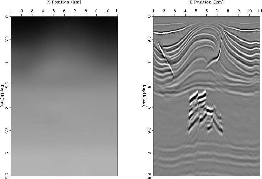
To test the methodology, I started with a fairly complex 2-D synthetic. The synthetic, shown in Figure 1, contains a realistic reservoir bounded by a faulted anticline and a basement rock. The velocity generally follows structure but with some low spatial frequency anomalies that range up to 5% of the background velocity. The synthetic reservoir is based on a real North Sea reservoir. The velocity and density structures vary significantly within the reservoir. The overburden was designed to break most conventional model characterization schemes. A layer-based approach would have difficulty with the anomalies and a gridded approach would find the sharp contrasts introduced by the faulting troublesome.

 

correct
Figure 1 A 2-D synthetic. A realistic reservoir bounded by a faulted anticline and a basement rock. The left panel shows the velocity, the panel is the result of migrating with the correct velocity.

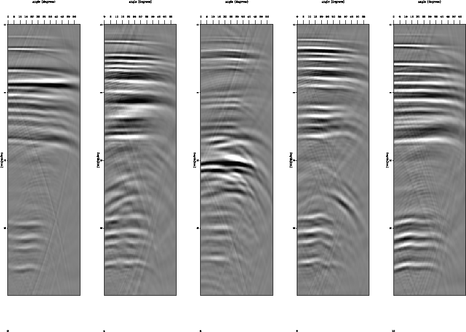
As an initial velocity estimate, I smoothed significantly the correct model. Figure 2 shows the initial velocity and the resulting migration. The basement reflectors are no longer flat and the anticline structure is more compressed in shape. The common reflection point gathers, five of which are shown in Figure 3, show significant move-out.

 

initial
Figure 2 The left panel shows the initial velocity model. The right panel shows the resulting of migrating with this velocity model.

 

gathers
Figure 3 Five CRP gathers (X=2,4,6,8,10) using the velocity shown in the left panel of Figure 2.

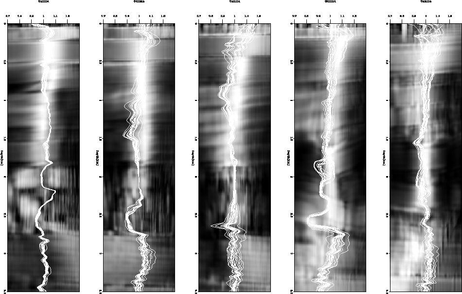
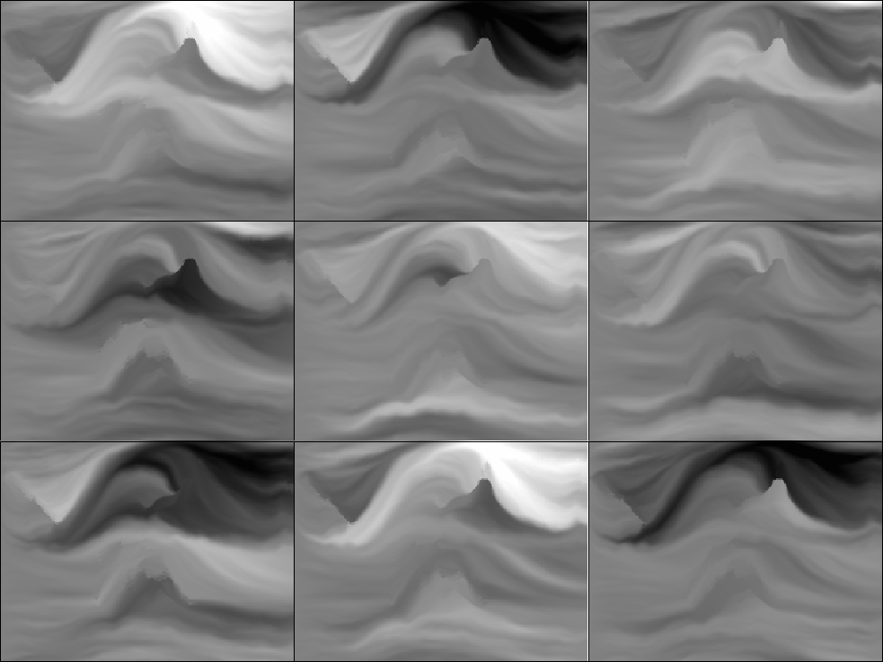
I then performed SRM semblance analysis on the dataset using $\gamma$ ranging from .7 to 1.3. Figure 4 shows the semblance scans for the same five locations as in Figure 3. I used the initial migration image to construct a steering filter for the colored random number generation. Figure 5 shows nine realizations of applying fitting goals (12). Note how the generated random numbers follow the image structure shown in Figure 2, but vary dramatically from realization to realization. I converted these random numbers to $\gamma$ values using cdfs generated at every location using equation (11). Thirty realizations of $\gamma$ values overlay the semblance scans in Figure 4. The various realizations are smooth as function of depth, which is reasonable. The amount of variance also seems reasonable. Note how when we have a sharp semblance maximum we see almost no variation, while when our blob is more spread out, the selected gamma values are more diverse. Note the fourth from the left gather at 1.8 seconds. Two different maxima are present in the semblance gather and we see that both are picked by various realizations. 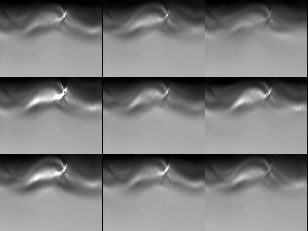Figure 6 shows nine gamma maps as a function of space. The $\gamma$ values are white when $\gamma=1$ and become more red has $\gamma$ becomes lower, and more blue as $\gamma$ increases. Note how we see a spatial consistency within a panel but differences between the panels. The top-right portion of the various realizations is especially interesting. We see $\gamma$ values greater than one, less than one, and some mix of both are selected by the various realizations.

 

picks
Figure 4 Five different SM semblance scans at the CRP locations shown in Figure 4. Overlaying the semblance scans are 30 different $\gamma$ realizations. Note the fourth from the left gather at 1.8 seconds. Two different maxims are present in the semblance gather and we see that both are picked by various realizations.

 

rand
Figure 5 Nine realizations of random numbers colored by applying fitting goals (12). Note how the random numbers follow geologic dip but vary significantly from image to image.

 

gamma_mult
Figure 6 Nine realizations of $\gamma$ values using the random numbers shown in Figure 5. Note how we see a spatial consistency within a panel but differences between the panels.

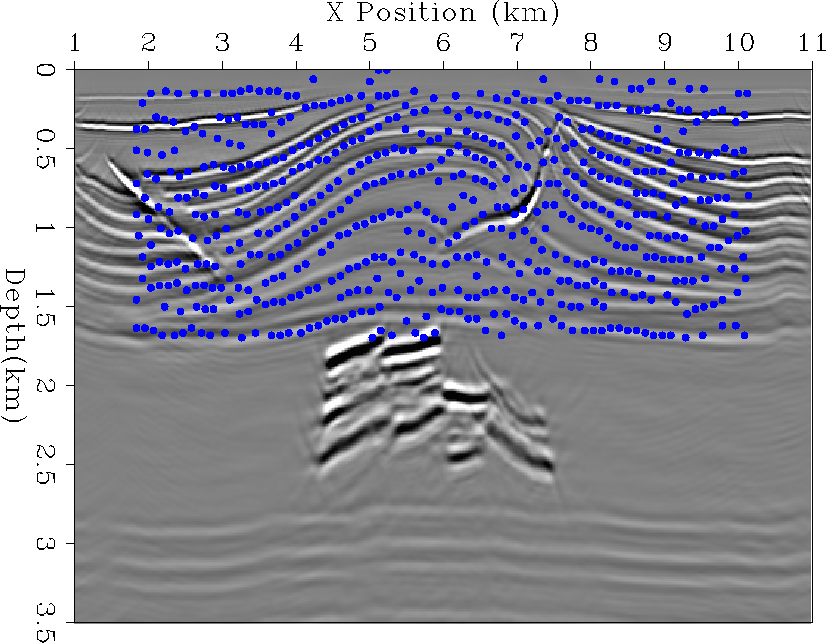
The $\gamma$ value were then used to update the velocity model using a preconditioned version of fitting goals (7). At this stage we are so far away from the correct answer that I limited the tomography to selecting back projection shallower than 1.7 km. Figure 7 shows the selected back projection points overlaid upon the migrated model. Figure 8 shows nine realizations of the tomography problem using the $\gamma$ values shown in Figure 6. Note the variance in the velocity structure from realization to realization. It is especially noticeable at the fault through the anticline and to the left the fault. We see velocity variations of 1 km/s or greater between the various realizations. This isn't surprising given the variance present in our semblance scans (Figure 4).

 

points Figure 7 The points used to update the velocity model using ray-based tomography overlaying the initial migrated image.

 

vel_mult
Figure 8 Nine realizations of tomography using the $\gamma$ values shown in Figure 6. Note the variation in the velocity structure especially to the left of the fault cutting through the anticline.

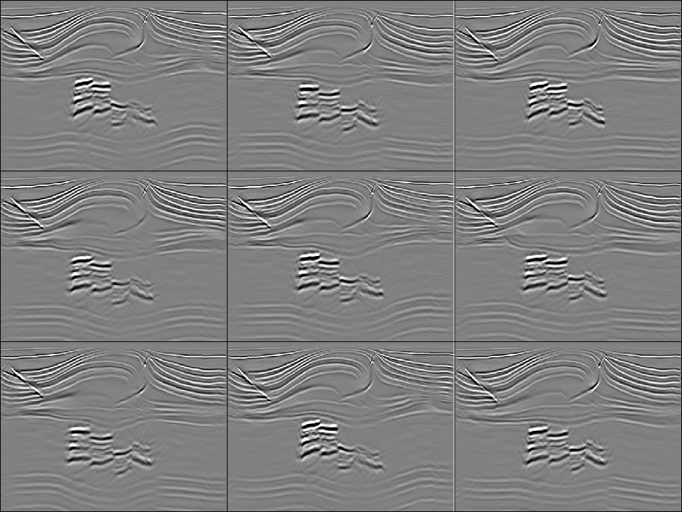
As a final step, I migrated the data with the various velocity models. Figure 9 shows the nine images corresponding to the nine velocity models shown in Figure 8. Note the differences in the various images. The top-right image shows a much flatter basement reflector than any of the other realizations. The variation in positioning of the fault reflector is also significant between the various realizations.

 

image_mult
Figure 9 Nine realizations corresponding to the nine velocity models shown in Figure 8. Note the differences in the various images. The top-right image shows a much flatter basement reflector than any of the other realizations. The variation positioning of the fault reflector is also significant between the various realizations.