Shot continuation

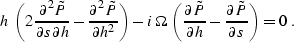
Missing or under-sampled shot records are a common example of data irregularity Crawley (2000). The offset continuation approach can be easily modified to work in the shot record domain. With the change of variables s = y - h, where s is the shot location, the frequency-domain equation () transforms to the equation  

$$h \, \left( 2\,{\partial^2 \tilde{P} \over \partial s \parti... ...h}} - {\partial \tilde{P} \over {\partial s}}\right) = 0 \;.$$ (133)

Unlike equation (), which is second-order in the propagation variable h, equation () contains only first-order derivatives in s. We can formally write its solution for the initial conditions at s=s₁ in the form of a phase-shift operator:  

$$\widehat{\widehat{P}}(s_2) = \widehat{\widehat{P}}(s_1)\, \... ...1\right)\, \frac{k_h\,h-\Omega}{2\,k_h\,h-\Omega}\right]}\;,$$ (134)

where the wavenumber k_h corresponds to the half-offset h. Equation () is in the mixed offset-wavenumber domain and, therefore, not directly applicable in practice. However, we can use it as an intermediate step in designing a finite-difference shot continuation filter. Analogously to the cases of plane-wave destruction and offset continuation, shot continuation leads us to the rational filter  

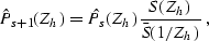$$\hat{P}_{s+1}(Z_h) = \hat{P}_{s} (Z_h) \frac{S(Z_h)}{\bar{S}(1/Z_h)}\;,$$ (135)

The filter is non-stationary, because the coefficients of S(Z_h) depend on the half-offset h. We can find them by the Taylor expansion of the phase-shift equation () around zero wavenumber k_h. For the case of the half-offset sampling equal to the shot sampling, the simplest three-point filter is constructed with three terms of the Taylor expansion. It takes the form  

$$S(Z_h) = - \left(\frac{1}{12} + i\,\frac{h}{2\,\Omega}\righ... ... i\,\frac{\Omega^2 + 18\,h^2}{12\,\Omega\,h}\right)\, Z_h\;.$$ (136)

Let us consider the problem of doubling the shot density. If we use two neighboring shot records to find the missing record between them, the problem reduces to the least-squares system  

$$\left[\begin{array} {c} \bold{S} \\ \bold{\bar{S}} \end{... ...{p}_{s-1} \\ \bold{S}\,\bold{p}_{s+1} \end{array}\right]\;,$$ (137)

where $\bold{S}$ denotes convolution with the numerator of equation (), $\bold{\bar{S}}$ denotes convolution with the corresponding denominator, $\bold{p}_{s-1}$ and $\bold{p}_{s+1}$ represent the known shot gathers, and $\bold{p}_s$ represents the gather that we want to estimate. The least-squares solution of system () takes the form  

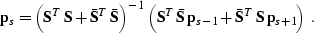$$\bold{p}_s = \left( \bold{S}^T\,\bold{S} + \bold{\bar{S}}... ...{s-1} + \bold{\bar{S}}^T\,\bold{S}\,\bold{p}_{s+1}\right)\;.$$ (138)

If we choose the three-point filter () to construct the operators $\bold{S}$ and $\bold{\bar{S}}$, then the inverted matrix in equation () will have five non-zero diagonals. It can be efficiently inverted with a direct banded matrix solver using the LDL^T decomposition Golub and Van Loan (1996). Since the matrix does not depend on the shot location, we can perform the decomposition once for every frequency so that only a triangular matrix inversion will be needed for interpolating each new shot. This leads to an extremely efficient algorithm for interpolating intermediate shot records.

Sometimes, two neighboring shot gathers do not fully constrain the intermediate shot. In order to add an additional constraint, I include a regularization term in equation (), as follows:  

$$\bold{p}_s = \left( \bold{S}^T\,\bold{S} + \bold{\bar{S}}... ...{s-1} + \bold{\bar{S}}^T\,\bold{S}\,\bold{p}_{s+1}\right)\;,$$ (139)

where $\bold{A}$ represents convolution with a three-point prediction-error filter (PEF), and $\epsilon$ is a scaling coefficient. The appropriate PEF can be estimated from $\bold{p}_{s-1}$ and $\bold{p}_{s+1}$ using Burg's algorithm Burg (1972, 1975); Claerbout (1976). A three-point filter leads does not break the five-diagonal structure of the inverted matrix. The PEF regularization attempts to preserve offset dip spectrum in the under-constrained parts of the estimated shot gather.

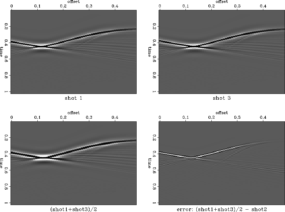
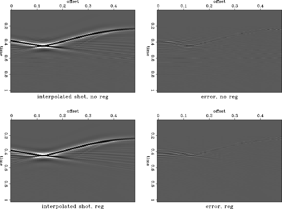
Figure  shows the result of a shot interpolation experiment using the constant-velocity synthetic from Figure . In this experiment, I removed one of the shot gathers from the original data and interpolated it back using equation (). Subtracting the true shot gather from the reconstructed one shows a very insignificant error, which is further reduced by using the PEF regularization (right plots in Figure ). The two neighboring shot gathers used in this experiment are shown in the top plots of Figure . For comparison, the bottom plots in Figure  show the simple average of the two shot gathers and its corresponding prediction error. As expected, the error is significantly larger than the error of the shot continuation. An interpolation scheme based on local dips in the shot direction would probably achieve a better result, but it is generally much more expensive than the shot continuation scheme introduced above.

 

shot3
Figure 38 Top: Two synthetic shot gathers used for the shot interpolation experiment. An NMO correction has been applied. Bottom: simple average of the two shot gathers (left) and its prediction error (right).

 

shotin
Figure 39 Synthetic shot interpolation results. Left: interpolated shot gathers. Right: prediction errors (the differences between interpolated and true shot gathers), plotted on the same scale. Top: without regularization. Bottom: with PEF regularization.

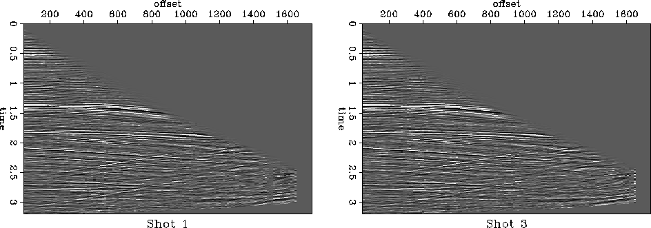
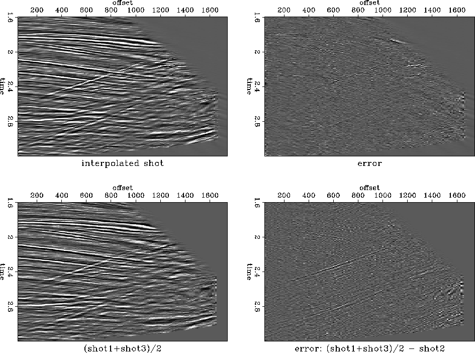
A similar experiment with real data from a North Sea marine dataset is reported in Figure . I removed and reconstructed a shot gather from the two neighboring gathers shown in Figure . The lower parts of the gathers are complicated by salt dome reflections and diffractions with conflicting dips. The simple average of the two input shot gathers (bottom plots in Figure ) works reasonably well for nearly flat reflection events but fails to predict the position of the back-scattered diffractions events. The shot continuation method works well for both types of events (top plots in Figure ). There is some small and random residual error, possibly caused by local amplitude variations.

 

elfshot3
Figure 40 Two real marine shot gathers used for the shot interpolation experiment. An NMO correction has been applied.

 

elfshotin
Figure 41 Real-data shot interpolation results. Top: interpolated shot gather (left) and its prediction error (right). Bottom: simple average of the two input shot gathers (left) and its prediction error (right).