3-D data regularization with the offset continuation equation

Similarly to the case of 3-D plane-wave destruction, where the regularization operator is constructed from two orthogonal two-dimensional filters, 3-D differential offset continuation amounts to applying two differential filters, operating on the in-line and cross-line projections of the offset and midpoint coordinates. The corresponding system of differential equations has the form  

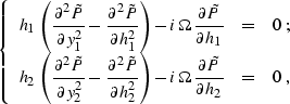$$\displaystyle \left\{\begin{array} {rcl} \displaystyle h... ... \tilde{P} \over {\partial h_2}} & = & 0\;, \end{array}\right.$$ (132)

where y₁ and y₂ correspond to the in-line and cross-line midpoint coordinates, and h₁ and h₂ correspond to the in-line and cross-line offsets. The projection approach is justified in the theory of azimuth moveout Biondi et al. (1998); Fomel and Biondi (1995b).

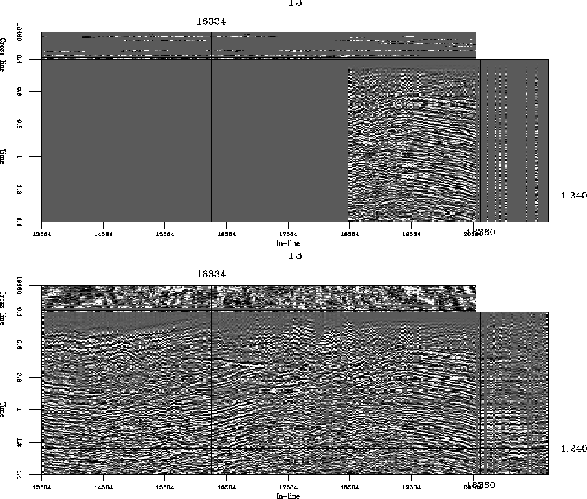
The result of a 3-D data regularization test is shown in Figure . The input data cube corresponds to the one in Figure . I used neighboring offsets in the in-line and cross-line directions and the differential 3-D offset continuation to reconstruct the empty traces. Although the reconstruction appears less accurate than the plane-wave regularization result of Figure , it successfully fulfills the following goals:

• The input traces are well hidden in the interpolation result. It is impossible to distinguish between input and interpolated traces.
• The main structural features are restored without using any assumptions about structural continuity in the midpoint domain. Only the physical offset continuity is used.

The lower accuracy of the result in Figure  in comparison with Figure  is partially caused by using a simplified missing data interpolation scheme instead of a more accurate regularization approach. It also indicates a possibility of combining offset continuation with midpoint-space plane-wave destruction for achieving an optimal accuracy.

 

off4
Figure 37 3-D data regularization test. Top: input data, the result of binning in a 50 by 50 meters offset window. Bottom: regularization output. Data from neighboring offset bins in the in-line and cross-line directions were used to reconstruct missing traces.

In the next section, I return to the 2-D case to consider an important problem of shot gather interpolation.