


Next: About this document ...
Up: Fomel: Offset continuation
Previous: RANGE OF VALIDITY FOR
In this appendix I derive formulas connecting second-order partial
derivatives of the reflection traveltime with the geometric properties
of the reflector in a constant velocity medium. These formulas are used in the
main text of the paper for the amplitude behavior description.
Let  be the reflection traveltime from the source s to the
receiver r. Consider a formal equality
be the reflection traveltime from the source s to the
receiver r. Consider a formal equality
|  |
(59) |
where x is the reflection point parameter,  corresponds to the
incident ray, and
corresponds to the
incident ray, and  corresponds to the reflected ray.
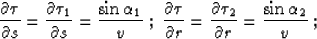
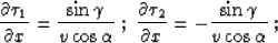
Differentiating (B-1) with respect to s and r yields
corresponds to the reflected ray.
Differentiating (B-1) with respect to s and r yields
| 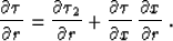 |
(60) |
|  |
(61) |
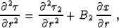
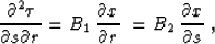
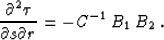
According to Fermat's principle, the two-point reflection ray path must
correspond to the traveltime extremum. Therefore
| 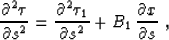 |
(62) |
for any s and r. Taking into account (B-4) while differentiating
(B-2) and (B-3), we get
|  |
(63) |
|  |
(64) |
|  |
(65) |
where
Differentiating (B-4) gives us the additional pair of equations
|  |
(66) |
|  |
(67) |
where
Solving the system (B-8) - (B-9) for  and
and
 and substituting the result into (B-5) -
(B-7)
produces the following set of expressions:
and substituting the result into (B-5) -
(B-7)
produces the following set of expressions:
|  |
(68) |
|  |
(69) |
|  |
(70) |
In the case of a constant velocity medium, expressions (B-10) to
(B-12) can be applied directly to the explicit
formula for the two-point eikonal
|  |
(71) |
Differentiating (B-13) and taking into account the trigonometric
relationships for the incident and reflected rays (Figure
1), one can
evaluate all the quantities in (B-10) to (B-12) explicitly.
After some heavy algebra, the resultant expressions for the traveltime
derivatives take the form
|  |
(72) |
|  |
(73) |
|  |
(74) |
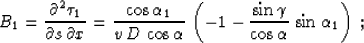
|  |
(75) |
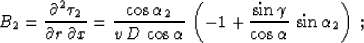
|  |
(76) |
| 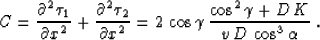 |
(77) |
|  |
(78) |
Here D is the length of the normal (central) ray,  is its dip angle
(
is its dip angle
( ,
,  ),
),
 is the reflection angle
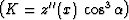 , K is the reflector
curvature at the reflection point , and
a is the nondimensional function of and defined in (35).
, K is the reflector
curvature at the reflection point , and
a is the nondimensional function of and defined in (35).
The formulas derived in this appendix were used to get the formula
|  |
(79) |
which coincides with (38) in the main text.
Next: About this document ...
Up: Fomel: Offset continuation
Previous: RANGE OF VALIDITY FOR
Stanford Exploration Project
6/19/2000