

Next: Beyond B-splines
Up: Forward Interpolation
Previous: B-splines
For completeness, I include a 2-D forward interpolation example.
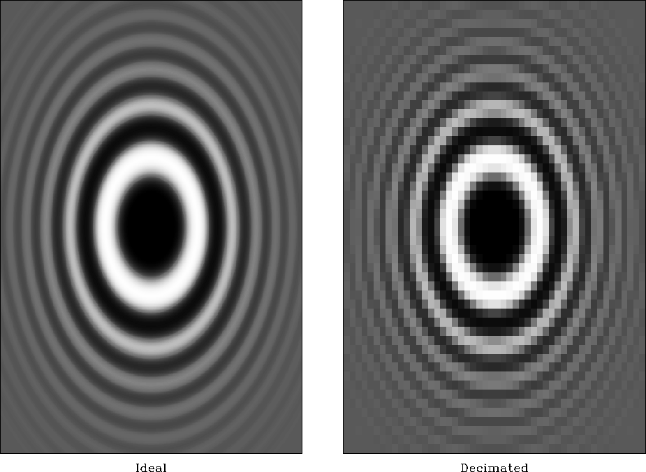
Figure ![[*]](http://sepwww.stanford.edu/latex2html/cross_ref_motif.gif) shows a 2-D analog of function in
Figure
shows a 2-D analog of function in
Figure ![[*]](http://sepwww.stanford.edu/latex2html/cross_ref_motif.gif) and its coarsely-sampled version.
chirp2
and its coarsely-sampled version.
chirp2
Figure 19 Two-dimensional test function
(left) and its coarsely sampled version (right).


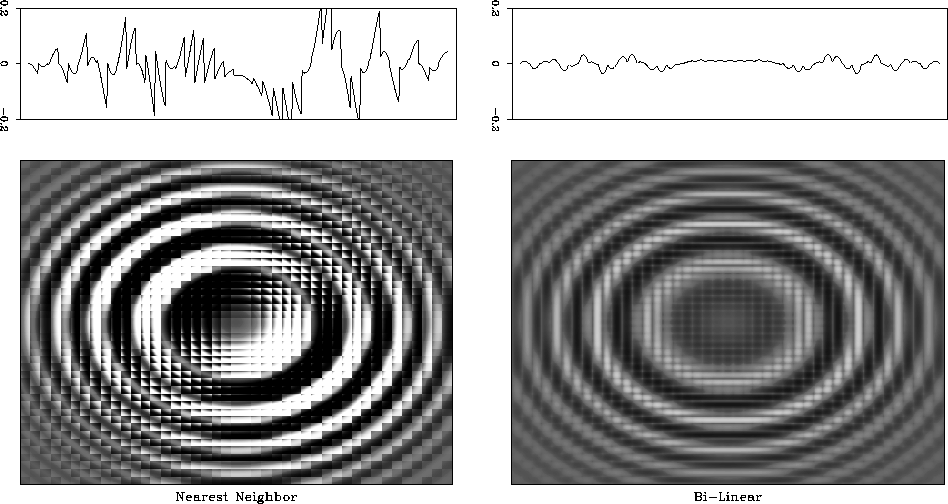
Figure ![[*]](http://sepwww.stanford.edu/latex2html/cross_ref_motif.gif) compares the errors of the 2-D nearest
neighbor and 2-D linear (bi-linear) interpolation. Switching to
bi-linear interpolation shows a significant improvement, but the error
level is still relatively high. As shown in
Figures
compares the errors of the 2-D nearest
neighbor and 2-D linear (bi-linear) interpolation. Switching to
bi-linear interpolation shows a significant improvement, but the error
level is still relatively high. As shown in
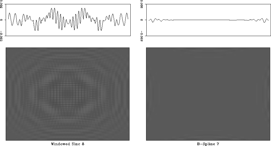
Figures ![[*]](http://sepwww.stanford.edu/latex2html/cross_ref_motif.gif) and
and ![[*]](http://sepwww.stanford.edu/latex2html/cross_ref_motif.gif) , B-spline
interpolation again outperforms other methods with comparable
cost complexity. In all cases, I constructed 2-D interpolants by orthogonal
splitting. Although the splitting method reduces computational
overhead, the main cost factor is the total interpolant size, which
squares when going from 1-D to 2-D.
, B-spline
interpolation again outperforms other methods with comparable
cost complexity. In all cases, I constructed 2-D interpolants by orthogonal
splitting. Although the splitting method reduces computational
overhead, the main cost factor is the total interpolant size, which
squares when going from 1-D to 2-D.
plcbinlin
Figure 20 2-D Interpolation errors of
nearest neighbor interpolation (left) and linear interpolation
(right). Top graphs show 1-D slices through the center of the
image.


 plccubspl
Figure 21 2-D Interpolation errors of
cubic convolution interpolation (left) and third-order B-spline
interpolation (right). Top graphs show 1-D slices through the
center of the image.


 plckaispl
Figure 22 2-D Interpolation errors of
8-point windowed sinc interpolation (left) and seventh-order
B-spline interpolation (right). Top graphs show 1-D slices through
the center of the images.


Next: Beyond B-splines
Up: Forward Interpolation
Previous: B-splines
Stanford Exploration Project
11/9/2000

![[*]](http://sepwww.stanford.edu/latex2html/cross_ref_motif.gif) shows a 2-D analog of function in
Figure
shows a 2-D analog of function in
Figure ![[*]](http://sepwww.stanford.edu/latex2html/cross_ref_motif.gif) and its coarsely-sampled version.
and its coarsely-sampled version.

![[*]](http://sepwww.stanford.edu/latex2html/cross_ref_motif.gif) compares the errors of the 2-D nearest
neighbor and 2-D linear (bi-linear) interpolation. Switching to
bi-linear interpolation shows a significant improvement, but the error
level is still relatively high. As shown in
Figures
compares the errors of the 2-D nearest
neighbor and 2-D linear (bi-linear) interpolation. Switching to
bi-linear interpolation shows a significant improvement, but the error
level is still relatively high. As shown in
Figures ![[*]](http://sepwww.stanford.edu/latex2html/cross_ref_motif.gif) and
and ![[*]](http://sepwww.stanford.edu/latex2html/cross_ref_motif.gif) , B-spline
interpolation again outperforms other methods with comparable
cost complexity. In all cases, I constructed 2-D interpolants by orthogonal
splitting. Although the splitting method reduces computational
overhead, the main cost factor is the total interpolant size, which
squares when going from 1-D to 2-D.
, B-spline
interpolation again outperforms other methods with comparable
cost complexity. In all cases, I constructed 2-D interpolants by orthogonal
splitting. Although the splitting method reduces computational
overhead, the main cost factor is the total interpolant size, which
squares when going from 1-D to 2-D.


