|
missif
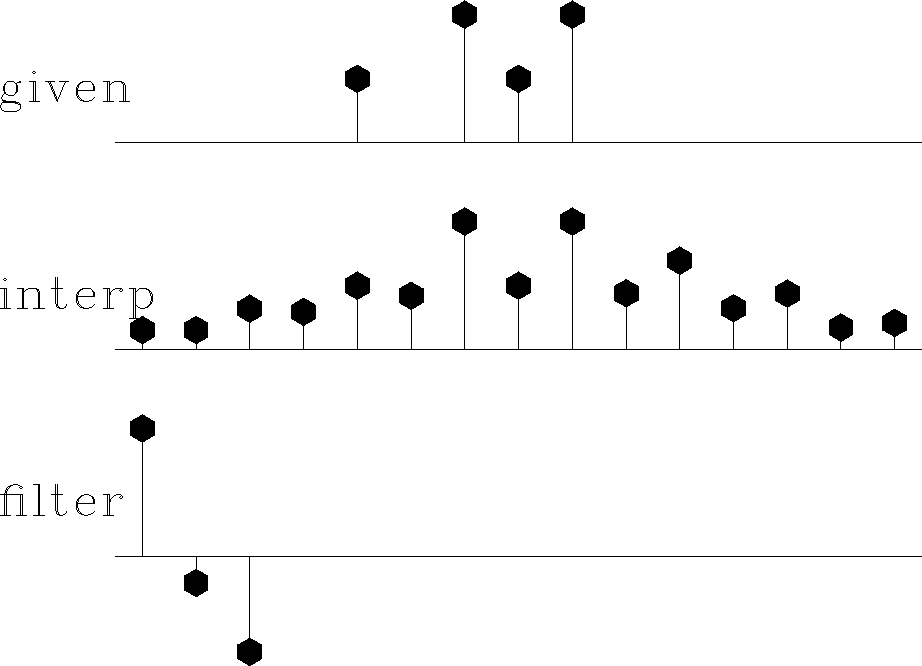
Figure 8 Top is known data. Middle includes the interpolated values. Bottom is the filter with the leftmost point constrained to be unity and other points chosen to minimize output power. |  |
In Figure 8 the filter is constrained to be of the form (1,a1,a2).
|
missif
Figure 8 Top is known data. Middle includes the interpolated values. Bottom is the filter with the leftmost point constrained to be unity and other points chosen to minimize output power. |  |
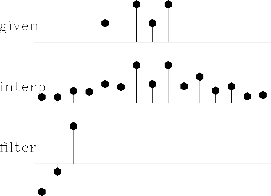
The result is pleasing in that the interpolated traces have the same general character as the given values. The filter came out slightly different from the (1,0,-1) that I suggested for Figure 7 based on a subjective analysis. Curiously, constraining the filter to be of the form (a-2,a-1,1) in Figure 9 yields the same interpolated missing data as in Figure 8. I understand that the sum squared of the coefficients of A(Z)P(Z) is the same as that of A(1/Z)P(Z), but I do not see why that would imply the same interpolated data.
|
backwards
Figure 9 The filter here had its rightmost point constrained to be unity--i.e., this filtering amounts to backward prediction. The interpolated data seems to be identical, as with forward prediction. |  |