


This paragraph describes only the false starts I made toward the solution.
It seems that the filter should be something like (1,-2,1),
because that filter interpolates on straight lines
and is not far from the feedback coefficients of a damped sinusoid.
(See equation (![[*]](http://sepwww.stanford.edu/latex2html/cross_ref_motif.gif) ).)
So I thought about different ways to force the solution
to move in that direction.
Traditional linear inverse theory offers several suggestions;
I puzzled over these before I found the right one.
First, I added the obvious stabilizations
).)
So I thought about different ways to force the solution
to move in that direction.
Traditional linear inverse theory offers several suggestions;
I puzzled over these before I found the right one.
First, I added the obvious stabilizations
![]() and
and
![]() ,but they simply made the filter and the interpolated data smaller.
I thought about changing the identity matrix in
,but they simply made the filter and the interpolated data smaller.
I thought about changing the identity matrix in ![]() to a diagonal matrix
to a diagonal matrix
![]() or
or
![]() .Using
.Using ![]() , I could penalize the filter
at even-valued lags, hoping that it
would become nonzero at odd lags, but that did not work.
Then I thought of using
, I could penalize the filter
at even-valued lags, hoping that it
would become nonzero at odd lags, but that did not work.
Then I thought of using
![]() ,
,![]() ,
,
![]() , and
, and
![]() ,which would allow freedom of choice of the mean and variance
of the unknowns.
In that case, I must supply
the mean and variance, however, and doing that seems
as hard as solving the problem itself.
Suddenly,
I realized the answer.
It is simpler than anything above,
yet formally it seems more complicated,
because a full inverse covariance matrix
of the unknown filter is implicitly supplied.
,which would allow freedom of choice of the mean and variance
of the unknowns.
In that case, I must supply
the mean and variance, however, and doing that seems
as hard as solving the problem itself.
Suddenly,
I realized the answer.
It is simpler than anything above,
yet formally it seems more complicated,
because a full inverse covariance matrix
of the unknown filter is implicitly supplied.
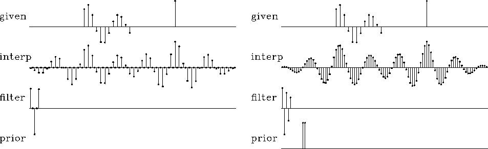
I found a promising new approach in the stabilized minimization
| |
(4) |
The next question is, what are the appropriate definitions for P0 and A0? Do we need both P0 and A0, or is one enough? We will come to understand P0 and A0 better as we study more examples. Simple theory offers some indications, however. It seems natural that P0 should have the spectrum that we believe to be appropriate for P. We have little idea about what to expect for A, except that its spectrum should be roughly inverse to P.
To begin with, I think of P0 as a low-pass filter, indicating that data is normally oversampled. Likewise, A0 should resemble a high-pass filter. When we turn to two-dimensional problems, I will guess first that P0 is a low-pass dip filter, and A0 a high-pass dip filter.
Returning to the one-dimensional signal-interlacing problem, I take A0=0 and choose P0 to be a different dataset, which I will call the ``training data.'' It is a small, additional, theoretical dataset that has no missing values. Alternately, the training data could come from a large collection of observed data that is without missing parts. Here I simply chose the short signal (1,1) that is not interlaced by zeros. This gives the fine solution we see in Figure 12.
 |


To understand the coding implied by
the optimization (4),
it is helpful to write the linearized regression.
The training signal P0 enters as a matrix of shifted columns
of the training signal, say ![]() ;and the high-pass filter A0 also appears
as shifted columns in a matrix, say
;and the high-pass filter A0 also appears
as shifted columns in a matrix, say ![]() .The unknowns A and P appear
both in the matrices
.The unknowns A and P appear
both in the matrices ![]() and
and ![]() and in vectors
and in vectors ![]() and
and ![]() .The linearized regression is
.The linearized regression is
![\begin{displaymath}
\left[
\begin{array}
{c}
-\bold P \bold a \
-\bold H \...
...y}
{c}
\Delta \bold p \
\Delta \bold a \end{array} \right]\end{displaymath}](img42.gif) |
(5) |
The top row restates equation (3).
The middle row says that
![]() ,and the bottom row says that
,and the bottom row says that
![]() .A program that does the job
is misfip() .
It closely resembles missif() .
.A program that does the job
is misfip() .
It closely resembles missif() .
# MISFIP -- find MISsing peF and Input data on 1-axis using Prior data.
#
subroutine misfip( nt,tt, na,aa, np,pp,known, niter)
integer nt, na,  ip,np,  npa, nta, nx,nr, iter,niter,  ax, px, qr, tr
real    pp(np), known(np), aa(na)       # same as in missif()
real    tt(nt)                          # input: prior training data set.
temporary real   x(np+na),             g(np+na),             s(np+na)
temporary real  rr(np+na-1 +na+nt-1), gg(np+na-1 +na+nt-1), ss(np+na-1 +na+nt-1)
npa= np+na-1;   nta= nt+na-1            # lengths of outputs of filtering
nx = np+na;     nr= npa+nta             # length of unknowns and residuals
px=1;           qr=1;   ax=1+np;        tr=1+npa        # pointers
call zero( na, aa);     aa(1) = 1.
call copy( np,  pp, x(px))
call copy( na,  aa, x(ax))
do iter= 0, niter {
        call contran( 0, 0, na,aa, np, pp,    rr(qr))
        call contran( 0, 0, na,aa, nt, tt,    rr(tr))  # extend rr with train
        call scaleit( -1.,           nr,        rr    )
        call contran( 1, 0, na,aa, np, g(px), rr(qr))
        call contran( 1, 0, np,pp, na, g(ax), rr(qr))
        call contran( 1, 1, nt,tt, na, g(ax), rr(tr))
        do ip= 1, np {  if( known(ip) != 0) { g( ip+(px-1)) = 0. } }
                                              g( 1 +(ax-1)) = 0.
        call contran( 0, 0, na,aa, np, g(px), gg(qr))
        call contran( 0, 1, np,pp, na, g(ax), gg(qr))
        call contran( 0, 0, nt,tt, na, g(ax), gg(tr))
        call cgstep( iter,  nx, x, g, s,  nr, rr, gg, ss)
        call copy( np, x(px), pp)
        call copy( na, x(ax), aa)
        }
return; end
The new computations are the lines containing the training data tt.
(I omitted the extra clutter of the high-pass filter hh
because I did not get an interesting example with it.)
Compared to missif() ,
additional clutter arises from pointers needed to partition
the residual and the gradient abstract vectors into three parts,
the usual one for || P A ||
and the new one for || P0 A ||
(and potentially ||P A0||).
You might wonder why we need
another program when we could use the old program
and simply append the training data to the observed data.
We will encounter some applications where
the old program will not be adequate.
These involve the boundaries of the data.
(Recall that, in chapter , when seismic events changed their dip,
we used a two-dimensional wave-killing operator
and were careful not to convolve the operator over the edges.)
Imagine a dataset that changes with time (or space).
Then P0 might not be training data,
but data from a large interval,
while P is data in a tiny window that is moved around on the big interval.
These ideas will take definite form in two dimensions.