An ideal bandpass filter passes some range of frequencies without distortion
and suppresses all other frequencies.
Further thought shows that what we think of as
the ideal bandpass filter,
a rectangle function of frequency,
is instead far from ideal, because its time-domain representation
![]() is noncausal and decays much too slowly with time for many practical uses.
The appropriate bandpass filter is one
whose time decay can be chosen to be reasonable
(in combination with a reasonable
necessary compromise on the shape of the rectangle).
Butterworth filters fulfill these needs.
is noncausal and decays much too slowly with time for many practical uses.
The appropriate bandpass filter is one
whose time decay can be chosen to be reasonable
(in combination with a reasonable
necessary compromise on the shape of the rectangle).
Butterworth filters fulfill these needs.
They are causal and of various orders, the lowest order being best (shortest) in the time domain, and the higher orders being better in the frequency domain. Well-engineered projects often include Butterworth filters. Unfortunately they are less often used in experimental work because of a complicated setting-up issue that I am going to solve for you here. I will give some examples and discuss pitfalls as well.
The main problem is that there is no simple mathematical expression for the filter coefficients as a function of order and cutoff frequency.
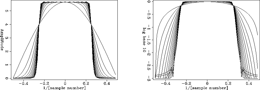
Analysis starts from an equation that for large-order n is the equation of a box:
 |
(21) |
 |
Conceptually, the easiest form of Butterworth filtering is to take data to the frequency domain and multiply by equation (21), where you have selected some value of n to compromise between the demands of the frequency domain (sharp cutoff) and the time domain (rapid decay). Of course, the time-domain representation of equation (21) is noncausal. If you prefer a causal filter, you could take the Butterworth spectrum into a spectral-factorization program such as kolmogoroff().
The time-domain response of the Butterworth filter is infinitely long,
although a Butterworth filter of degree n
can be well approximated by a ratio of ![]() -order polynomials.
Since, as we will see,
n is typically in the range 2-5,
time-domain filtering is quicker than FT.
To proceed, we need to express
-order polynomials.
Since, as we will see,
n is typically in the range 2-5,
time-domain filtering is quicker than FT.
To proceed, we need to express ![]() in terms of Z,
where
in terms of Z,
where ![]() .This is done in an approximate way that is valid for frequencies
far from the Nyquist frequency.
Intuitively we know that time differentiation is implied by
.This is done in an approximate way that is valid for frequencies
far from the Nyquist frequency.
Intuitively we know that time differentiation is implied by ![]() .We saw that in sampled time,
differentiation is generally represented by the bilinear transform,
equation (
.We saw that in sampled time,
differentiation is generally represented by the bilinear transform,
equation (![[*]](http://sepwww.stanford.edu/latex2html/cross_ref_motif.gif) ):
):
![]() .Thus a sampled-time representation
of
.Thus a sampled-time representation
of ![]() is
is
| |
(22) |
![\begin{eqnarray}
B \left( {1 \over Z} \right) B(Z)
&=&
{[ (1+Z^{-1})(1+Z)]^n \ov...
... {1 \over Z} \right) B(Z)
&=&
{N(Z^{-1})N(Z) \over D(Z^{-1}) D(Z)}\end{eqnarray}](img86.gif) |
(23) | |
| (24) |