The hope method

We have examined the two-stage linear method of missing-data restoration, which calls for solving for a filter, interlacing it, and then solving for the missing data. I believe that method, with its interlacing, is unsuitable for data with a narrow spectral signal-to-noise ratio, such as we often encounter in practice. It would indeed be nice to be able to work with such data.

Recall equation (4):

$$\min_{P,A} \ \ (\vert\vert P A \vert\vert \ +\ \lambda_9 \v... ... A \vert\vert \ +\ \lambda_{10} \vert\vert P A_0 \vert\vert \ )$$

Now we hope to solve the trace-interlace problem directly from this optimization. Without the training data P₀ and the high-pass filter A₀, however, the trace-interlace problem is highly nonlinear, and, as in the case of the one-dimensional problem, I found I was unable to descend to a satisfactory solution. Therefore, we must think about what the training data and prior filter might be. Our first guess might be that P₀ is a low-pass dip filter and A₀ is a high-pass dip filter. Several representations for low- and high-pass dip filters are described in IEI. I performed a few tests with them but was not satisfied with the results.

Another possibility is that P₀ should be the solution as found by the interlacing method. Time did not allow me to investigate this promising idea.

Still another possibility is that these problems are so easy to solve (requiring workstation compute times of a few seconds only) that we should abandon traditional optimization methods and use simulated annealing (Rothman, 1985).

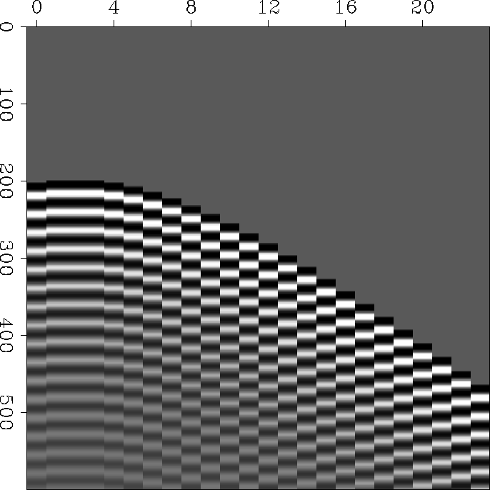
All the above ideas are hopeful. A goal of this study is to define and characterize the kinds of problems that we think should be solvable. A simple example of a dataset that I believe should be amenable to interpolation, even with substantial noise, is shown in Figure 22. I have not worked with this case yet.

 

alias Figure 22 Narrow-banded data that skilled humans can readily interpolate.

To prepare the way, and to perform my preliminary (but unsatisfactory) tests, I prepared subroutine hope(), the two-dimensional counterpart to missif() and misfip() . 

subroutine hope( gap, h1,h2,hh, t1,t2,tt, a1,a2,aa, p1,p2,pp, known, niter)
integer         h1,h2,h12,  t1,t2,t12,  a1,a2,a12,  p1,p2,p12
integer         i, gap, iter, niter, midpt, nx,nr, px,ax,  qr,tr,hr
real            hh(h1,h2), tt(t1,t2), aa(a1,a2), pp(p1*p2), known(p1*p2), dot
temporary real  x( p1*p2 +a1*a2),  rr( p1*p2 +p1*p2 +t1*t2)
temporary real  g( p1*p2 +a1*a2),  gg( p1*p2 +p1*p2 +t1*t2)
temporary real  s( p1*p2 +a1*a2),  ss( p1*p2 +p1*p2 +t1*t2)
p12 = p1*p2;    a12 = a1*a2;    t12 = t1*t2;    h12= h1*h2;
nx  = p12 + a12;          px= 1;        ax= 1+p12
nr  = p12 + p12 + t12;    qr= 1;        hr= 1+p12;      tr= 1+p12+p12
call zero( a12, aa);    midpt= a1/2;    aa( midpt, 1 ) = sqrt( dot( p12,pp,pp))
call zero( nx, x);      call zero( nr, rr);     call copy( p12, pp, x(px))
call zero( nx, g);      call zero( nr, gg);     call copy( a12, aa, x(ax))
do iter= 0, niter {
        call cinloi( 0, 0, midpt,1, a1,a2,aa, p1,p2,pp,    rr(qr))
        call cinloi( 0, 0, midpt,1, h1,h2,hh, p1,p2,pp,    rr(hr))
        call cinloi( 0, 0, midpt,1, a1,a2,aa, t1,t2,tt,    rr(tr))
        call scaleit (                     -1., nr,          rr    )
        call cinloi( 1, 0, midpt,1, a1,a2,aa, p1,p2,g(px), rr(qr))
        call cinlof( 1, 0, midpt,1, p1,p2,pp, a1,a2,g(ax), rr(qr))
        call cinloi( 1, 1, midpt,1, h1,h2,hh, p1,p2,g(px), rr(hr))
        call cinlof( 1, 1, midpt,1, t1,t2,tt, a1,a2,g(ax), rr(tr))
        do i= 1, p12       { if( known(i) != 0.)    g( i + (px-1)) = 0.}
        do i= 1, midpt+gap {                        g( i + (ax-1)) = 0.}
        call cinloi( 0, 0, midpt,1, a1,a2,aa, p1,p2,g(px), gg(qr))
        call cinlof( 0, 1, midpt,1, p1,p2,pp, a1,a2,g(ax), gg(qr))
        call cinloi( 0, 0, midpt,1, h1,h2,hh, p1,p2,g(px), gg(hr))
        call cinlof( 0, 0, midpt,1, t1,t2,tt, a1,a2,g(ax), gg(tr))
        call cgstep( iter, nx,  x, g, s, _
                           nr, rr,gg,ss )
        call copy( p12, x(px), pp)
        call copy( a12, x(ax), aa)
        }
return; end

I found the jump-and-interlace 2-D convolution cinjof() unsuitable here because it does not align its output consistently with the aligning convolution cinloi() . So I wrote an aligning convolution identical with cinloi() except that the filter is the adjoint. It is called cinlof(). 

# CINLOF -- Convolution INternal with Lags.  Output is adjoint to FILTER.
#
subroutine cinlof( adj, add, lag1,lag2,  n1,n2,xx,  nb1,nb2,bb,  yy)
integer            adj, add, lag1,lag2,  n1,n2,     nb1,nb2
real                                      xx(n1,n2), bb(nb1,nb2), yy(n1,n2)
integer y1,y2, x1,x2, b1, b2
call adjnull(      adj, add,                         bb,nb1*nb2,  yy,n1*n2)
if( adj == 0 )
        do b2=1,nb2 { do y2= 1+nb2-lag2, n2-lag2+1 {  x2= y2 - b2 + lag2
        do b1=1,nb1 { do y1= 1+nb1-lag1, n1-lag1+1 {  x1= y1 - b1 + lag1
                                yy(y1,y2) = yy(y1,y2) + bb(b1,b2) * xx(x1,x2)
                                }} }}
else
        do b2=1,nb2 { do y2= 1+nb2-lag2, n2-lag2+1 {  x2= y2 - b2 + lag2
        do b1=1,nb1 { do y1= 1+nb1-lag1, n1-lag1+1 {  x1= y1 - b1 + lag1
                                bb(b1,b2) = bb(b1,b2) + yy(y1,y2) * xx(x1,x2)
                                }} }}
return; end