


What is a truly
two-dimensional prediction-error filter?![[*]](http://sepwww.stanford.edu/latex2html/foot_motif.gif) This is a question we should answer
in our quest to understand resonant signals
aligned along various dips.
Figure 11 shows that
an interpolation-error filter is no substitute for a PE filter
in one dimension.
So we need to use special care
in properly defining a 2-D PE filter.
Recall the basic proof in chapter
This is a question we should answer
in our quest to understand resonant signals
aligned along various dips.
Figure 11 shows that
an interpolation-error filter is no substitute for a PE filter
in one dimension.
So we need to use special care
in properly defining a 2-D PE filter.
Recall the basic proof in chapter ![[*]](http://sepwww.stanford.edu/latex2html/cross_ref_motif.gif) (page ) that
the output of a PE filter is white.
The basic idea is that the output residual is uncorrelated
with the input fitting functions (delayed signals); hence,
by linear combination,
the output is uncorrelated with the past outputs
(because past outputs are also linear combinations of past inputs).
This is proven for one side of the autocorrelation,
and the last step in the proof is to note that what is true
for one side of the autocorrelation must be true for the other.
Therefore, we need to extend the idea of ``past'' and ``future'' into
the plane to divide the plane into two halves.
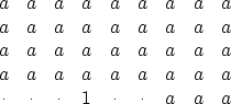
Thus I generally take a 2-D PE filter to be of the form
(page ) that
the output of a PE filter is white.
The basic idea is that the output residual is uncorrelated
with the input fitting functions (delayed signals); hence,
by linear combination,
the output is uncorrelated with the past outputs
(because past outputs are also linear combinations of past inputs).
This is proven for one side of the autocorrelation,
and the last step in the proof is to note that what is true
for one side of the autocorrelation must be true for the other.
Therefore, we need to extend the idea of ``past'' and ``future'' into
the plane to divide the plane into two halves.
Thus I generally take a 2-D PE filter to be of the form
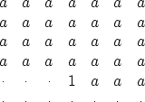 |
(12) |
The three-dimensional prediction-error filter
which embodies the same concept is shown in Figure 21.
|
3dpef
Figure 21 Three-dimensional prediction-error filter. | 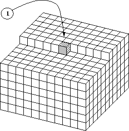 |

Can ``short'' filters be used?
Experience shows that a significant detriment to whitening with a PE
filter
is an underlying model that is not purely a polynomial division
because it has a convolutional (moving average) part.
The convolutional part is especially troublesome
when it involves serious bandlimiting,
as does convolution with bionomial coefficients
(for example, the Butterworth filter, discussed in chapter ).
When bandlimiting occurs,
it seems best to use a gapped PE filter.
I have some limited experience with 2-D PE filters that suggests using a gapped form like
 |
(13) |
.
Explain how to do the job properly.