

Next: MARINE DEGHOSTING
Up: Model fitting by least
Previous: Preconditioning
Starting from a hypothetical, ideal,
zero-offset model,
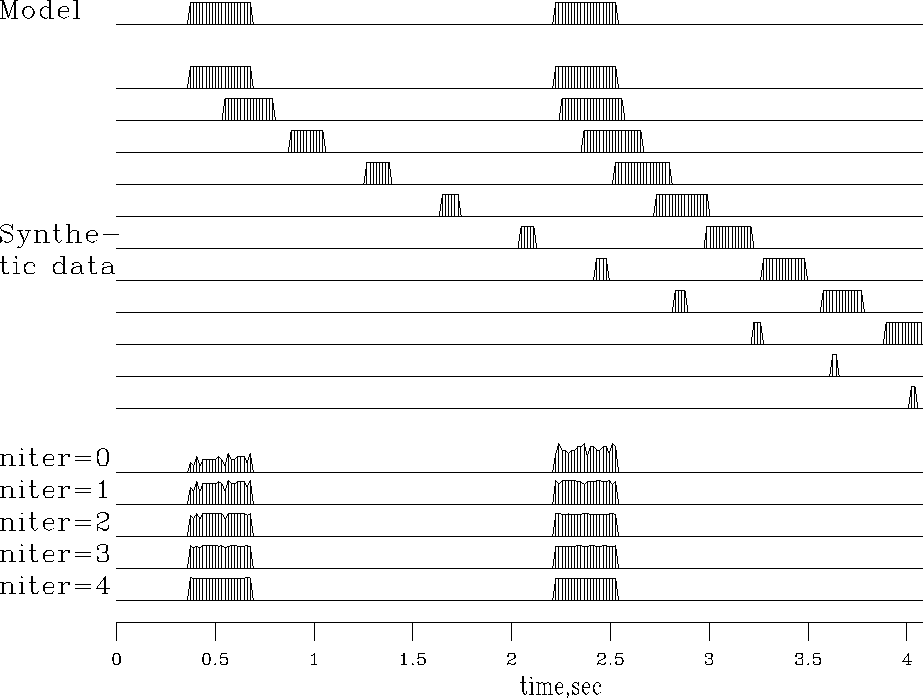
Figure ![[*]](http://sepwww.stanford.edu/latex2html/cross_ref_motif.gif) shows synthetic data
and the result of adjoint modeling (back projection),
which reconstructs an imperfect model.
Inversion should enable us to reconstruct the original model.
Let us see how
back projection can be upgraded towards
inversion.
shows synthetic data
and the result of adjoint modeling (back projection),
which reconstructs an imperfect model.
Inversion should enable us to reconstruct the original model.
Let us see how
back projection can be upgraded towards
inversion.
Unfortunately,
the adjoint operator  defined by the subroutine nmo1()
 ![[*]](http://sepwww.stanford.edu/latex2html/cross_ref_motif.gif) is not a good operator for seismogram modeling--notice
the roughness of the synthetic seismograms
in Figure
is not a good operator for seismogram modeling--notice
the roughness of the synthetic seismograms
in Figure ![[*]](http://sepwww.stanford.edu/latex2html/cross_ref_motif.gif) .
This roughness is not an inevitable consequence
of nearest-neighbor interpolation.
It is a consequence of defining the NMO program as a loop
over the output space
.
This roughness is not an inevitable consequence
of nearest-neighbor interpolation.
It is a consequence of defining the NMO program as a loop
over the output space  .Instead,
we can define inverse NMO
as a loop over its output space,
which is not
  but t.
This is done in imo1()
 ![[*]](http://sepwww.stanford.edu/latex2html/cross_ref_motif.gif) and imospray()
and imospray() ![[*]](http://sepwww.stanford.edu/latex2html/cross_ref_motif.gif) .
.
|
If we plan an upgrade from back projection
towards inversion,
we must be aware that the accuracy of the original modeling
operator can become an issue.
|


The new seismograms at the bottom of Figure 1
show the first four iterations of conjugate-gradient inversion.
You see the original rectangle-shaped waveform returning
as the iterations proceed.
Notice also on the stack
that the early and late events have unequal amplitudes,
but after iteration they are equal,
as they began.
Mathematically,
we can denote the top trace as the model  ,the synthetic data signals as
  ,and the stack as
  .The conjugate-gradient algorithm solves the regression
 by variation of
  ,and the figure shows
  converging to
  .Since there are 256 unknowns in
  ,it is gratifying to see good convergence occurring
after the first four iterations.
The CG subroutine used is invstack(),
which is just like
cgmeth()
 ![[*]](http://sepwww.stanford.edu/latex2html/cross_ref_motif.gif) except that the matrix-multiplication operator
matmul()
except that the matrix-multiplication operator
matmul() ![[*]](http://sepwww.stanford.edu/latex2html/cross_ref_motif.gif) has been replaced by
imospray()
has been replaced by
imospray() ![[*]](http://sepwww.stanford.edu/latex2html/cross_ref_motif.gif) .
Studying the program,
you can deduce that,
except for a scale factor,
the output at niter=0 is identical to the stack
.
Studying the program,
you can deduce that,
except for a scale factor,
the output at niter=0 is identical to the stack  .All the signals in Figure 1 are intrinsically the same scale.
# NMO stack by inverse of forward modeling
#
subroutine invstack(  nt,model,nx,gather,rr,t0,x0,dt,dx,slow,niter)
integer it, ix, iter, nt,      nx,                           niter
real    t0,x0,dt,dx,slow, gather(nt,nx), rr(nt,nx), model(nt)
temporary real  dmodel(nt), smodel(nt), dr(nt,nx), sr(nt,nx)
do it= 1, nt
        model(it) = 0.0
do it= 1, nt
        do ix= 1, nx
                rr(it,ix) = gather(it,ix)
do iter = 0, niter {
        call imospray( 1,0,slow,x0,dx,t0,dt,nx,nt,dmodel,rr)    # nmo-stack
        call imospray( 0,0,slow,x0,dx,t0,dt,nx,nt,dmodel,dr)    # modeling
        call cgstep(iter,   nt, model, dmodel, smodel, _
	                 nt*nx, rr,    dr,     sr)
        }
return; end
This simple inversion is inexpensive.
Has anything been gained over conventional stack?
First,
though we used nearest-neighbor interpolation,
we managed to preserve the spectrum of the input,
apparently all the way to the Nyquist frequency.
Second, we preserved the true amplitude scale
without ever bothering to think about
(1) dividing by the number of contributing traces,
(2) the amplitude effect of NMO stretch, or
(3) event truncation.
With depth-dependent velocity,
wave fields become much more complex at wide offset.
NMO soon fails,
but wave-equation forward modeling
offers interesting opportunities for inversion.


Next: MARINE DEGHOSTING
Up: Model fitting by least
Previous: Preconditioning
Stanford Exploration Project
10/21/1998
![[*]](http://sepwww.stanford.edu/latex2html/cross_ref_motif.gif) is not a good operator for seismogram modeling--notice
the roughness of the synthetic seismograms
in Figure
is not a good operator for seismogram modeling--notice
the roughness of the synthetic seismograms
in Figure ![[*]](http://sepwww.stanford.edu/latex2html/cross_ref_motif.gif) .
This roughness is not an inevitable consequence
of nearest-neighbor interpolation.
It is a consequence of defining the NMO program as a loop
over the output space
.
This roughness is not an inevitable consequence
of nearest-neighbor interpolation.
It is a consequence of defining the NMO program as a loop
over the output space ![[*]](http://sepwww.stanford.edu/latex2html/cross_ref_motif.gif) and imospray()
and imospray() ![[*]](http://sepwww.stanford.edu/latex2html/cross_ref_motif.gif) .
.
