Analytical approximations of p_h

Although the numerical solutions are sufficient and efficient enough to perform prestack migration, analytical solutions are important for obtaining insights into the problem. Analytical solutions are also important for inversion purposes where we need to calculate the solution and its derivatives for different medium parameters in an iterative fashion.

For homogeneous isotropic media, the stationary point is given by  

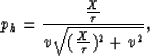
$$p_h = \frac{\frac{X}{\tau}}{v \sqrt{(\frac{X}{\tau})^2 + v^2}} (1-p_x^2 v^2)^{3/2} [a(p_{hs})p_x+1]$$ (19)

(Appendix B), where

$$a= \frac{1}{p_{h0} (1-p_x^2 v^2)^{3/2}} - \frac{1}{p_{hs}}.$$

and p_h0 and p_hs are given in the Appendix. This equation is obtained by fitting p_h to it's exact solution at three different values of p_x, and therefore, I will refer to it as the 3-point solution. For p_x=0, although not directly obvious, equation (19) reduces to

$$p_h = \frac{\frac{X}{\tau}}{v \sqrt{(\frac{X}{\tau})^2 + v^2}},$$

which corresponds to the exact stationary point solution for horizontal reflectors. As demonstrated in Appendix B, this equation can be extracted directly from the hyperbolic moveout relation for a homogeneous isotropic medium. The other two terms in equation (19), the ones in circular and square brackets, insure that we obtain the exact solution of the stationary point at p_x=p_h, and $p_x=\frac{1}{v}$,respectively.

The 2-point solution, shown in Appendix B, is the same as equation (19) without the term in square brackets. As a result, this equation fits the exact solution at p_x=0 and $p_x=\frac{1}{v}$, and, therefore, I will refer to it as the 2-point solution. The low curvature of T around its maximum (see Figure 1) makes any error attributed to equation (19) or to the 2-point solution to be insignificant, even for large offsets.

The stationary point solutions for homogeneous VTI media are much more complicated, as shown in Appendix B, than their isotropic counterparts. Nevertheless, they have the same form (2- and 3-point fitting solutions) as that for isotropic media. The solutions for p_x=0 and p_x=p_h, however, are no longer exact because we dropped some terms (related to strong anisotropy and large offsets) in their derivation. Nevertheless, the approximations, as shown in Appendix B and in the following subsection, are relatively accurate. In fact, using the perturbation theory along with Shanks transforms, one can obtain even better approximations of p_h (see Appendix C).