

Next: Marmousi velocity model
Up: EXAMPLES
Previous: Constant velocity
The velocity model I now consider has a constant gradient, with both the
vertical and horizontal velocity gradients equal to 1.0 km/s/km.
The dimensions are the same as the previous constant velocity model.
In this case, the velocity ranges linearly from 1.0 km/s in the upper
left corner to 13 km/s in the lower right corner, which is an extremely
strong gradient compared to what may be naturally observed.
I presume that we have two previously calculated traveltime fields
at surface source positions of x = 2.75 km and 3.25 km, i.e., a
sparse traveltime table sampling every 500 m along the line (my other
rule of thumb goal in addition to beating 1% relative error).
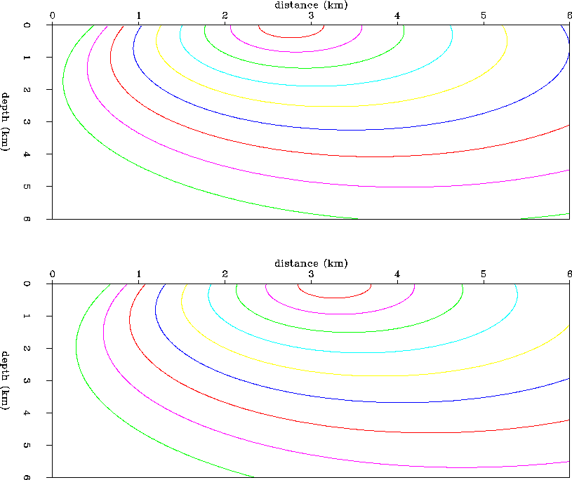
Figure ![[*]](http://sepwww.stanford.edu/latex2html/cross_ref_motif.gif) shows the contours of traveltime due to the source at 2.75 km (upper panel),
and due to a source at 3.25 km (lower panel). Since I interpolate
traveltime gradients, and not the traveltimes themselves, Figures
shows the contours of traveltime due to the source at 2.75 km (upper panel),
and due to a source at 3.25 km (lower panel). Since I interpolate
traveltime gradients, and not the traveltimes themselves, Figures
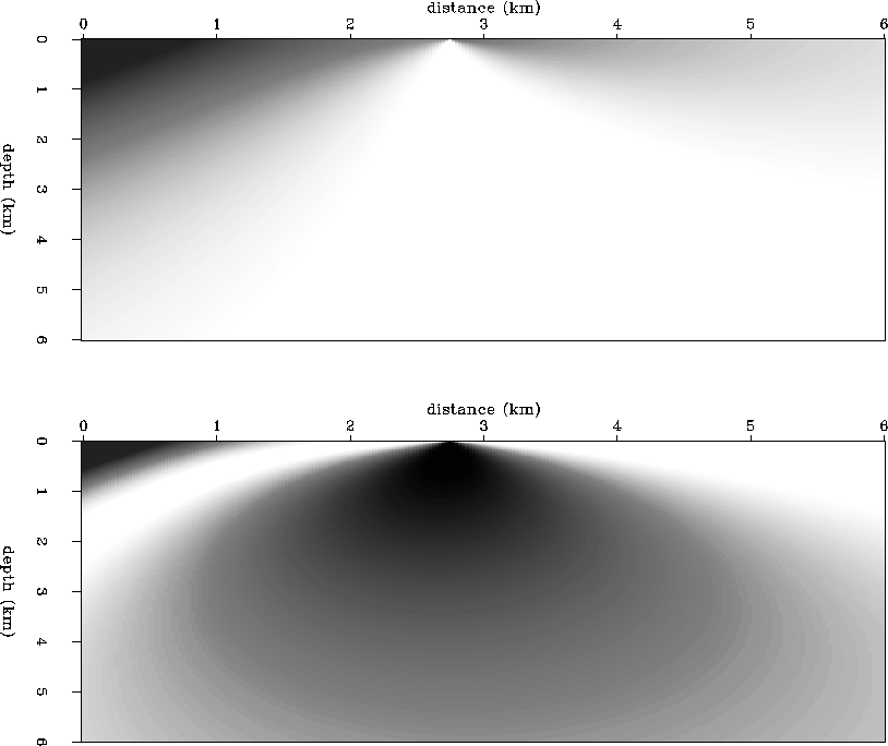
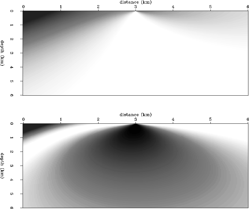
![[*]](http://sepwww.stanford.edu/latex2html/cross_ref_motif.gif) shows the horizontal and vertical traveltime gradients
shows the horizontal and vertical traveltime gradients
 and
and  for the first source position, and Figure
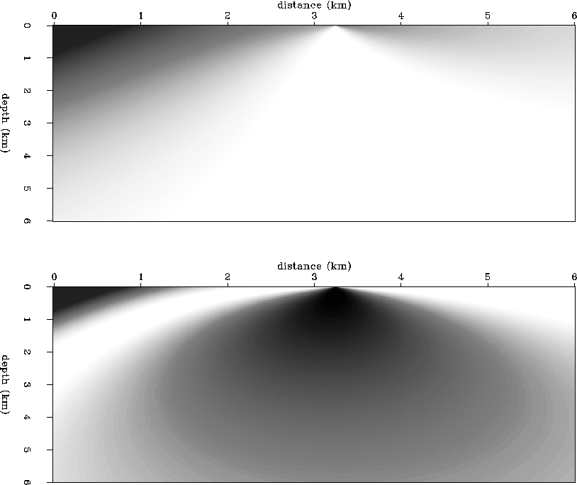
 ![[*]](http://sepwww.stanford.edu/latex2html/cross_ref_motif.gif) shows the
shows the  and
and  for the source given at 3.25 km.
I then solve system (13) using a combination of Cramer's Rule
where nonsingular, and Singular Value Decomposition otherwise.
I also use the cosine estimate and correction discussed previously
from (8) and (17).
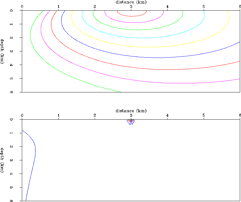
The interpolated traveltime field is shown in the upper panel of
Figure ![[*]](http://sepwww.stanford.edu/latex2html/cross_ref_motif.gif) for
a desired surface source position at 3.0 km. The lower panel of
Figure
for
a desired surface source position at 3.0 km. The lower panel of
Figure ![[*]](http://sepwww.stanford.edu/latex2html/cross_ref_motif.gif) shows the relative error between the interpolated traveltime field,
and the true traveltime field obtained by an analytic raytracing algorithm
for constant gradient velocity media (Zhang, 1992, pers. comm.).
The error contours are at 1% farthest from the source region, and
increase to 10% in the near vicinity of the source. The interpolation
is highly accurate, except for some small error directly beneath the
source position. This is caused by the previously mentioned
instability at the source
position in the vertical traveltime gradient, and it is propagated
somewhat into all of the traveltimes by the subsequent spatial integration.
To help stabilize the singularity,
I calculate the
shows the relative error between the interpolated traveltime field,
and the true traveltime field obtained by an analytic raytracing algorithm
for constant gradient velocity media (Zhang, 1992, pers. comm.).
The error contours are at 1% farthest from the source region, and
increase to 10% in the near vicinity of the source. The interpolation
is highly accurate, except for some small error directly beneath the
source position. This is caused by the previously mentioned
instability at the source
position in the vertical traveltime gradient, and it is propagated
somewhat into all of the traveltimes by the subsequent spatial integration.
To help stabilize the singularity,
I calculate the  values within a few mesh
points of the source location by assuming straight rays (constant velocity)
from the source.
Figure
 ![[*]](http://sepwww.stanford.edu/latex2html/cross_ref_motif.gif) shows the interpolated horizontal
and vertical traveltime gradients respectively.
shows the interpolated horizontal
and vertical traveltime gradients respectively.
g13t
Figure 7 Linear gradient velocity model.
Contours of traveltime field for
the two given surface source positions at 2.75 km (top) and 3.25 km
(bottom).


 g1xz
g1xz
Figure 8 Linear gradient velocity model.
Horizontal (top) and vertical
(bottom) traveltime gradient fields for
the surface source positioned at 2.75 km.


 g3xz
g3xz
Figure 9 Linear gradient velocity model.
Horizontal (top) and vertical
(bottom) traveltime gradient fields for
the surface source positioned at 3.25 km.


 gite
gite
Figure 10 Linear gradient velocity model.
Interpolated traveltime field.
The top panel is the interpolated traveltime field for a surface
source positioned at 3.00 km. The lower panel is the relative
error between the interpolated traveltime field, and the correct
traveltimes modeled by an analytical solution to the eikonal. The
contour farthest from the source region is at 1% relative error,
and the contour values increase to 10% error right at the source
location, in 1% contour increments.


 gixz
gixz
Figure 11 Linear gradient velocity model.
Horizontal (top) and vertical
(bottom) traveltime gradient fields for
the interpolated surface source positioned at 3.00 km.


Next: Marmousi velocity model
Up: EXAMPLES
Previous: Constant velocity
Stanford Exploration Project
11/17/1997
![[*]](http://sepwww.stanford.edu/latex2html/cross_ref_motif.gif) shows the contours of traveltime due to the source at 2.75 km (upper panel),
and due to a source at 3.25 km (lower panel). Since I interpolate
traveltime gradients, and not the traveltimes themselves, Figures
shows the contours of traveltime due to the source at 2.75 km (upper panel),
and due to a source at 3.25 km (lower panel). Since I interpolate
traveltime gradients, and not the traveltimes themselves, Figures
![[*]](http://sepwww.stanford.edu/latex2html/cross_ref_motif.gif) shows the horizontal and vertical traveltime gradients
shows the horizontal and vertical traveltime gradients
![[*]](http://sepwww.stanford.edu/latex2html/cross_ref_motif.gif) shows the
shows the 