Now suppose I know a set of n Green's function traveltime fields
![]() for n source positions
for n source positions ![]() .
Estimating the traveltime field
.
Estimating the traveltime field ![]() ,
due to a single intermediate
surface source position
,
due to a single intermediate
surface source position ![]() , from the n given fields
, from the n given fields ![]() ,
is defined as traveltime interpolation.
,
is defined as traveltime interpolation.
For the set of ![]() , (7) can be generalized to a linear matrix
equation of the form:
, (7) can be generalized to a linear matrix
equation of the form:
| |
(12) |
or into a general weighted least-squares system ![]() :
:
 |
(13) |
System (13) can be solved by standard damped least-squares,
| |
(14) |
or by the optimal (but slow) Singular Value Decomposition (SVD)
method, for the components of the unknown vector ![]() .I refer the reader to Strang (1980) for an excellent review of damped
least squares and SVD linear algebra techniques.
The diagonal weighting matrix
.I refer the reader to Strang (1980) for an excellent review of damped
least squares and SVD linear algebra techniques.
The diagonal weighting matrix ![]() is of
dimensions (nxn), and the weights wi could be inverse-distance:
is of
dimensions (nxn), and the weights wi could be inverse-distance:
![]() ,
for example. The
,
for example. The ![]() matrix is (nx3) in 3-D and (nx2) in 2-D (ignoring
the
matrix is (nx3) in 3-D and (nx2) in 2-D (ignoring
the ![]() terms), and contains the vector components of the known traveltime
gradient fields. The data vector
terms), and contains the vector components of the known traveltime
gradient fields. The data vector ![]() is (nx1) and contains the
is (nx1) and contains the
![]() values. For a 2-D geometry, at least two traveltime
gradient fields must be known, and for a 3-D interpolation at least three
traveltime gradient fields must be available.
values. For a 2-D geometry, at least two traveltime
gradient fields must be known, and for a 3-D interpolation at least three
traveltime gradient fields must be available.
In the case of interpolation, a refinement to the estimate of the
![]() values is possible. In this paper, I use the Law of
Cosines given by (8) as an initial estimate of, say,
values is possible. In this paper, I use the Law of
Cosines given by (8) as an initial estimate of, say,
![]() and
and ![]() , where the traveltime field
at
, where the traveltime field
at ![]() is to be interpolated from two bounding source locations
is to be interpolated from two bounding source locations
![]() and
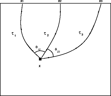
and ![]() . Please refer to Figure
. Please refer to Figure ![[*]](http://sepwww.stanford.edu/latex2html/cross_ref_motif.gif) to consider the
appropriate interpolation geometry.
However, the angle
to consider the
appropriate interpolation geometry.
However, the angle ![]() is known precisely from
the given traveltime (gradient) fields at
is known precisely from
the given traveltime (gradient) fields at ![]() and
and ![]() :
:
| |
(15) |
Therefore, given the angle estimates ![]() ,
, ![]() and
and
![]() , and the true angle
, and the true angle ![]() , I can refine my
initial (primed) estimates such that the total angle
, I can refine my
initial (primed) estimates such that the total angle ![]() is
conserved as a sum of
is
conserved as a sum of ![]() ,
, ![]() :
:
| |
(16) |
Then, the correction factor f is given as
![]()
| |
(17) |
As an example,
for a 2-D interpolation of ![]() given
given ![]() and
and ![]() , I first
set up a 2x2 matrix system per (13). I evaluate the required
data vector values
, I first
set up a 2x2 matrix system per (13). I evaluate the required
data vector values ![]() and
and ![]() using (8),
and refine the cosine estimates using (17). I then invert system
(13) by Cramer's Rule if the determinant is not too small, or by
SVD if otherwise. The entire procedure is repeated in a point-by-point
independent manner, making it an obvious candidate for massively parallel
implementation, for all subsurface grid locations
using (8),
and refine the cosine estimates using (17). I then invert system
(13) by Cramer's Rule if the determinant is not too small, or by
SVD if otherwise. The entire procedure is repeated in a point-by-point
independent manner, making it an obvious candidate for massively parallel
implementation, for all subsurface grid locations ![]() .
.
Finally, the traveltime gradients are spatially integrated to traveltime such that, for a source at (x2,z2) on a flat surface z = z2,
| |
(18) |
| |
(19) |
where H is the Heaviside function. This process completes
the traveltime interpolation of ![]() from
from ![]() and
and ![]() .
.
 |