The major problems in constructing model weighting functions occur in areas where strong aliased events cross weak unaliased events. The aliases of high energy events can be given low weights if they lie within the ``pass window'' of a lower energy event or alternatively a low energy event can lie within a ``reject region'' produced by a strong alias. One way to avoid this problem is to produce a initial estimate of the spectrum that has had the aliases of the high energy events predicted and removed.
I can use the ``masked'' slant stack method to create an estimate of
the ![]() spectrum that contains only events that are continuous
in frequency and high amplitude. I do this by designing a mask
function using a high value for the energy damping factor,
spectrum that contains only events that are continuous
in frequency and high amplitude. I do this by designing a mask
function using a high value for the energy damping factor, ![]() , in
the continuity estimator. Given this information I can subtract the
aliases of this energy from the initial estimate of the spectrum to
give an improved estimate.
, in
the continuity estimator. Given this information I can subtract the
aliases of this energy from the initial estimate of the spectrum to
give an improved estimate.
The aliases are estimated by assuming that the mask function selects
only unaliased energy. This data is then transformed to the ![]() domain at the original spacing and then back to the
domain at the original spacing and then back to the ![]() domain
using the simple transpose operator; using the transpose operator will
give a dataset with the aliased and unaliased events. The masking
function is then used to remove the unaliased events leaving only the
aliases of the high energy events.
domain
using the simple transpose operator; using the transpose operator will
give a dataset with the aliased and unaliased events. The masking
function is then used to remove the unaliased events leaving only the
aliases of the high energy events.
This improved estimate is now used as the
initial estimate of the solution in the iterative solver.
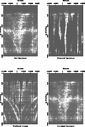
Figure ![[*]](http://sepwww.stanford.edu/latex2html/cross_ref_motif.gif) shows four stages in the estimation of the
improved initial estimate. The frames show the original data, the
windowed data which is assumed to contain strong, unaliased events,
the estimate of the aliases of the strong events, and finally the
improved initial estimate of the
shows four stages in the estimation of the
improved initial estimate. The frames show the original data, the
windowed data which is assumed to contain strong, unaliased events,
the estimate of the aliases of the strong events, and finally the
improved initial estimate of the ![]() spectrum.
spectrum.
 |
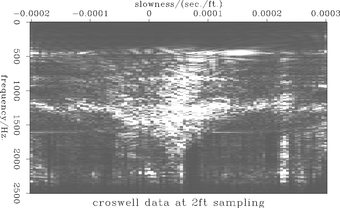
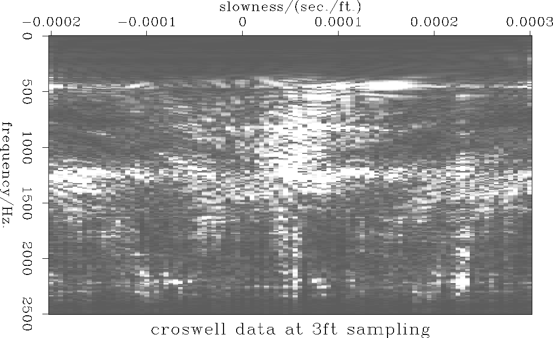
The least-squares estimate of the ![]() spectrum generated from
this improved estimate is displayed in figure
spectrum generated from
this improved estimate is displayed in figure ![[*]](http://sepwww.stanford.edu/latex2html/cross_ref_motif.gif) the
equivalent panel for the data samples at a 3ft. interval is displayed
in figure
the
equivalent panel for the data samples at a 3ft. interval is displayed
in figure ![[*]](http://sepwww.stanford.edu/latex2html/cross_ref_motif.gif) . Both are similar to the original spectrum
calculated from the data at a 1ft. sample interval
(figure
. Both are similar to the original spectrum
calculated from the data at a 1ft. sample interval
(figure ![[*]](http://sepwww.stanford.edu/latex2html/cross_ref_motif.gif) ). The detailed amplitudes are
slightly different but on both plots almost all the aliased
energy has been suppressed.
). The detailed amplitudes are
slightly different but on both plots almost all the aliased
energy has been suppressed.
 |
 |
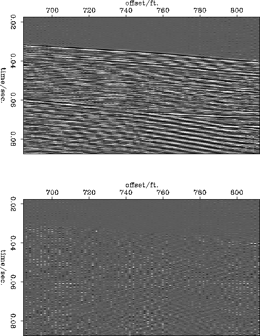
Figure ![[*]](http://sepwww.stanford.edu/latex2html/cross_ref_motif.gif) shows the data at 2ft. reconstructed at a 1ft
spacing and the difference between that and the original data at a
1ft. spacing. Figure
shows the data at 2ft. reconstructed at a 1ft
spacing and the difference between that and the original data at a
1ft. spacing. Figure ![[*]](http://sepwww.stanford.edu/latex2html/cross_ref_motif.gif) shows the same figures for the
data subsampled to a 3ft. spacing. The reconstruction from the 2ft
data is satisfactory. The main differences appear to be trace-to-trace
amplitude changes which were lost in the original subsampling and some
energy dipping to the left which was outside the slowness range
modeled in the slant stack data. The reconstruction from the 3ft. data
is obviously worse but it still retains the major features of the
original data and it does not contain any aliased data.
shows the same figures for the
data subsampled to a 3ft. spacing. The reconstruction from the 2ft
data is satisfactory. The main differences appear to be trace-to-trace
amplitude changes which were lost in the original subsampling and some
energy dipping to the left which was outside the slowness range
modeled in the slant stack data. The reconstruction from the 3ft. data
is obviously worse but it still retains the major features of the
original data and it does not contain any aliased data.
 |
 |