


Next: Fundamental solutions
Up: 4: CONNECTION WITH RAY
Previous: Ray method
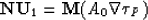
Let us consider the equation (32) for n = 0:

With accordance to equation (23), this is a linear algebraic
equation with degenerate matrices. It may be solved only in
the case when  is an eigenvector.
We restrict ourselves with the situation when the eiconal
equation for P-waves is valid. In this case, the eigenvector is
is an eigenvector.
We restrict ourselves with the situation when the eiconal
equation for P-waves is valid. In this case, the eigenvector is
 so vector can be
expressed in the form
so vector can be
expressed in the form  . In
order to specify the amplitude A0 let us consider the
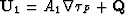
equation (32) for n = 1:
. In
order to specify the amplitude A0 let us consider the
equation (32) for n = 1:
|  |
(34) |
But any vector  can be decomposed into the sum
 where
where  . Both vectors
  and
and  are eigenvectors connected with eigenvalues
and
are eigenvectors connected with eigenvalues
and  correspondently, therefore,

We see that the left side of the equation (34) is
orthogonal to the vector . It means that
equation (33) can be resolved if and only if
| 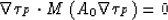 |
(35) |
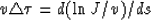
Inserting expression in equation (33) into the last equation, we use the
property of the operator , if s is the
natural parameter of a ray  , then for
any scalar function
, then for
any scalar function 
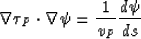
where ![$d[\cdot]/ds$](img226.gif) means differentiation along the ray that
intersects the given point. After simple manipulation we
derive from equation (35) the transient equation for the amplitude
A = A0/v:
means differentiation along the ray that
intersects the given point. After simple manipulation we
derive from equation (35) the transient equation for the amplitude
A = A0/v:
| ![\begin{displaymath}
\frac{dA}{ds} + \frac{1}{2}A[v \triangle \tau_{P} + \frac{
d (\ln \rho {v_P}^2)}{ds}] = 0\end{displaymath}](img227.gif) |
(36) |
which have solution
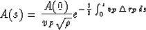
The well-known notion of geometrical spreading  is connected with
  by relation
(S.V. Goldin, 1986)
by relation
(S.V. Goldin, 1986)
consequently,
| 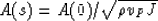 |
(37) |
Analogous formula is true for S-waves.
The equation (37) describes how the amplitude of the senior
discontinuity of a wave is changing along a ray path.
If the value of J is positive in all points of a given ray , then along the ray
| ![\begin{displaymath}
{\bf U} \sim \frac{A(0)}{\sqrt{\rho v_{P} {J}
}}R_{q_{0}} [t - t(s)]{\bf t}\end{displaymath}](img233.gif) |
(38) |
where ![$t(s) = \tau_{P}[{\bf r}(s)]$](img234.gif) and
and  is the tangent-vector of the ray. And
if J < 0, then
is the tangent-vector of the ray. And
if J < 0, then
![\begin{displaymath}
{\bf U} \sim \frac{A(0)}{\sqrt{\rho v_{P}{J}}}
R_{q_{0}, 1}[t - t(s)]{\bf t}\end{displaymath}](img236.gif)
The situation when J = 0 means that  at q'<q0,
  .
.
Next: Fundamental solutions
Up: 4: CONNECTION WITH RAY
Previous: Ray method
Stanford Exploration Project
1/13/1998