Methodology

Constraints were first applied to the flattening problem in Lomask and Guitton (2006). In the 3D Gauss-Newton flattening approach, data is flattened by iterating over the following equations iterate {

$$\begin{eqnarray} \bf r \quad &=& \quad [\boldsymbol{\nabla}_\epsilon \boldsymbol... ... &=& \quad \boldsymbol{\tau}_{k}(x,y,t) + \Delta \boldsymbol{\tau}\end{eqnarray}$$ (1) (2) (3)

} ,
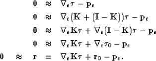
where the subscript k denotes the iteration number, $\boldsymbol{\tau}$ is the estimated time-shift found in the least-squares sense so that its gradient matches the dip ${\bf p}$, and $\epsilon$ is an adjustable regularization controlling the amount of conformity in the time (or depth) dimension. $\boldsymbol{\nabla}_\epsilon$ is a 3D gradient operator with an $\epsilon$ parameter. The residual update in equation (1) can be rewritten as  

$$\bf r \quad = \quad { \boldsymbol{\nabla}_\epsilon \boldsymb... ...} {c}{{\bf b}} \\ {{\bf q}} \\ {\bf 0} \end{array} \right] }.$$ (4)

I wish to add a model mask $\bf K$ to prevent changes to specific areas of an initial $\boldsymbol{\tau}_0$ field. This initial $\boldsymbol{\tau}_0$ field can be picks from any source. In general, they may come from a manually picked horizon or group of horizons. These initial constraints do not have to be continuous surfaces but instead could be isolated picks, such as well-to-seismic ties. To apply the mask I follow a similar development to Claerbout (1999) as

$$\begin{eqnarray} \bold 0 &\approx& \boldsymbol{\nabla}_\epsilon \boldsymbol{\ta... ...}_\epsilon\bold K\boldsymbol{\tau} + \bold r_0 - {\bf p}_\epsilon.\end{eqnarray}$$ (5) (6) (7) (8) (9)

The resulting equations are now iterate {

$$\begin{eqnarray} \bf r \quad &=& \quad \boldsymbol{\nabla}_\epsilon {\bf K}\bold... ...bol{\boldsymbol{\tau}}_{k} + \Delta \boldsymbol{\boldsymbol{\tau}}\end{eqnarray}$$ (10) (11) (12)

} .

Because the mask $\bf K$ in equation (11) is non-stationary, I solve it using preconditioned conjugate gradients. The preconditioner efficiently exploits Discrete Cosine Transforms(DCTs) to invert a Laplacian operator Lomask and Fomel (2006) as:  

$$\Delta \boldsymbol{\tau} \approx {\rm DCT_{3D}}^{-1} \left[{... ...abla_\epsilon\it{^{\rm T}}{\bf r} \right]}\ \over { J} \right],$$ (13)

where ${\rm DCT_{3D}}$ is the 3D discrete cosine transform and  

$$J= -2(\cos( w \Delta x)+\cos( w \Delta y)) +2\epsilon^2(1-\cos(w \Delta t))+4.$$ (14)

J is the real component of the Z-transform of the 3D finite difference approximation to the Laplacian with adjustable regularization.

Following an approach for weighted 2D phase unwrapping by Ghiglia and Romero (1994), I define ${\bold Q}={\bf K}^{\rm T} \boldsymbol{\nabla}_\epsilon^{\rm T}\boldsymbol{\nabla}_\epsilon{\bf K}$ and $\mathbf{ \bar r}={\bf K}^{\rm T} \boldsymbol{\nabla}_\epsilon^{\rm T}{\bf r}$ so that equation (11) becomes

$$\Delta \boldsymbol{\boldsymbol{\tau}} \quad =\quad {\bold Q}^{-1}{\bf \bar{r}}.$$ (15)

For each non-linear Gauss-Newton iteration, the least-squares solution to equation (11) is solved by iterating over the following preconditioned conjugate gradients computation template:

 

		 iterate { 
		 		 solve  ${\bold z}_k \quad = \quad (\boldsymbol{\nabla}_\epsilon^{\rm T}\boldsymbol{\nabla}_\epsilon)^{-1}\mathbf{ \bar r}_k$ using equation (13)
		 		 subtract off reference trace  ${\bold z}_k \quad = \quad {\bold z}_k-{\bold z}_k(ref)$ 
		 		 if first iteration {
		 		 		 ${\bold p}_1 \quad\longleftarrow\quad{\bold z}_0$ 
		 		 } else{
		 		 		 $\beta_{k+1} \quad\longleftarrow\quad\mathbf{ \bar r}_{k}^{\rm T}{\bold z}_k/\mathbf{ \bar r}_{k-1}^{\rm T}{\bold z}_{k-1}$ 
		 		 		 ${\bold p}_{k+1} \quad\longleftarrow\quad{\bold z}_k+\beta_{k+1}{\bold p}_{k}$ 
		 		 		 }
		 		 $\alpha_{k+1} \quad\longleftarrow\quad\mathbf{ \bar r}_{k}^{\rm T}{\bold z}_k/{\bold p}_{k+1}^{\rm T}{\bold Q}{\bold p}_{k+1}$ 
		 		 $\Delta \boldsymbol{\boldsymbol{\tau}}_{k+1} \quad\longleftarrow\quad\Delta \boldsymbol{\boldsymbol{\tau}}_k+\alpha_{k+1}{\bold p}_{k+1}$ 
		 		  $\mathbf{ \bar r}_{k+1} \quad\longleftarrow\quad\mathbf{ \bar r}_{k}-\alpha_{k+1}{\bold Q}{\bold p}_{k+1}$ 
		 		 } 

Here, k is the iteration number starting at k=0. It is necessary to subtract off the reference trace at each iteration because the Fourier based solution using equation (13) has no non-stationary information such as the location of the reference trace. Subtracting the reference trace removes a zero frequency shift. Nonetheless, in practice equation (13) makes an adequate preconditioner because $\boldsymbol{\nabla}_\epsilon^{\rm T}\boldsymbol{\nabla}_\epsilon$ is often close to ${\bf K}^{\rm T} \boldsymbol{\nabla}_\epsilon^{\rm T}\boldsymbol{\nabla}_\epsilon{\bf K}$.

Convergence can be determined using the same criterion described in Lomask et al. (2006). Alternatively, an adequate stopping criterion would be to consider only the norm of the residual $\Vert\mathbf{ \bar r}_{k}\Vert$. This is essentially the average of the divergence of the remaining dips, i.e. ,  

$${\frac{\Vert\mathbf{ \bar r}_{k}\Vert}{n}} \quad < \quad {\mu} ,$$ (16)

where $n=n_1 \times n_2 \times n_3$ is the size of the data cube.

 

• Constrained solution with weights